Estimated Burden of Bladder Cancer in the United States and Its States, 1990–2021: A Descriptive Analysis of the Global Burden of Disease (GBD) Study 2021

Alireza Sadeghi; Fatemeh Nouri; Niloofar Dehdari Ebrahimi; Ehsan Taherifard; Mohammadreza Soltani; Stephen B. Williams; Wassim Kassouf

In [1]:

.body-justified p {
  text-align: justify
}

In [2]:

# ---------------------------------------------------------------------------
# Set-up, data loading and helper functions
# ---------------------------------------------------------------------------

options(
  tidyverse.quiet = TRUE,
  dplyr.summarise.inform = FALSE
)

library(tidyverse)
library(scales)


Attaching package: 'scales'

The following object is masked from 'package:purrr':

    discard

The following object is masked from 'package:readr':

    col_factor

library(glue)
library(geofacet)
library(ggnewscale)
library(future)
library(furrr)
library(gganimate)

No renderer backend detected. gganimate will default to writing frames to separate files
Consider installing:
- the `gifski` package for gif output
- the `av` package for video output
and restarting the R session

library(paletteer)
library(flextable)


Attaching package: 'flextable'

The following object is masked from 'package:purrr':

    compose

# All files in data/ are GBD 2021 extracts from the GHDx GBD Results Tool.
# Only bladder cancer is analysed here (filter is defensive: the data folder
# should already contain only this cause).
bladder_data <- 
  list.files("data", "rds", full.names = TRUE) %>%
  map_df(read_rds, .progress = TRUE) %>% 
  bind_rows() %>% 
  filter(cause_name == "Bladder cancer")

 ■■■■■■■■■■■■■■■                   48% |  ETA:  2s

# Location IDs of the 50 states + District of Columbia (not a state; referred to
# as "jurisdictions" when pooled)
stateids <- 
  bladder_data %>% 
  filter(location_level == "United States of America") %>% 
  distinct(location_id) %>%
  pull(location_id)

source("scripts/functions.r")

# GBD location IDs used throughout
us_id <- 102
comp_ids <- c(us = 102, eu = 4743, hi = 64, hs = 44635)
region_labels <- c(
  "102" = "United States", 
  "4743" = "European Union", 
  "64" = "High-income", 
  "44635" = "High SDI"
)
keep_ids <- c(stateids, comp_ids)

# Age-standardized rates (metric "Rate", age_id 27) for U.S., states and comparators
asr <- 
  bladder_data %>% 
  filter(
    metric_id == 3, 
    age_id == 27, 
    location_id %in% keep_ids
  )

measure_label <- c(
  Incidence = "incidence", Prevalence = "prevalence", Deaths = "mortality",
  YLDs = "YLDs", YLLs = "YLLs", DALYs = "DALYs"
)

In [3]:

# ---------------------------------------------------------------------------
# Helper functions (these supersede ratio_calc()/diff_calc() in functions.r,
# which were called with swapped/transformed arguments in the first version)
# ---------------------------------------------------------------------------

# Number formatting: one decimal everywhere unless stated otherwise
fmt_num <- function(x, d = 1) scales::number(x, accuracy = 10^-d, big.mark = ",")
fmt_signed <- function(x, d = 1) {
  scales::number(x, accuracy = 10^-d, style_positive = "plus", style_negative = "minus")
}
# estimate [lower, upper]
fmt_ui  <- function(est, lo, hi, d = 1) {
  paste0(fmt_num(est, d), " [", fmt_num(lo, d), ", ", fmt_num(hi, d), "]")
}
# signed percent change with approximate UI: +x% [+l%, +u%]  (always lower, then upper)
fmt_pct <- function(est, lo, hi, d = 1) {
  paste0(fmt_signed(est, d), "% [", fmt_signed(lo, d), "%, ", fmt_signed(hi, d), "%]")
}

# Return exactly one row or fail loudly (avoids silent index-based mistakes)
pick <- function(data, ...) {
  out <- dplyr::filter(data, ...)
  if (nrow(out) != 1) stop("pick(): expected 1 row, got ", nrow(out), call. = FALSE)
  out
}

# Ratio of two estimates with approximate 95% UI, computed on the log scale.
# SE(log estimate) is back-calculated from the published UI bounds assuming the
# UI is symmetric on the log scale; the two estimates are assumed independent.
# Arguments are (estimate, LOWER, UPPER) for each quantity, in that order.
log_ratio_ui <- function(est1, lo1, hi1, est2, lo2, hi2, level = 0.95) {
  z <- qnorm(1 - (1 - level) / 2)
  se1 <- (log(hi1) - log(lo1)) / (2 * z)
  se2 <- (log(hi2) - log(lo2)) / (2 * z)
  se  <- sqrt(se1^2 + se2^2)
  lr  <- log(est1) - log(est2)
  tibble(
    ratio = est1 / est2,
    ratio_lower = exp(lr - z * se),
    ratio_upper = exp(lr + z * se)
  )
}

# Percent change of age-standardized rates between two years, for every
# measure x location x sex in `data`; percent change = 100 * (rate_y1 / rate_y0 - 1)
pct_change <- function(data, y0, y1) {
  wide <- 
    data %>% 
    filter(year %in% c(y0, y1)) %>% 
    mutate(period = if_else(year == y0, "start", "end")) %>% 
    select(
      measure_id, measure_name, location_id, location_name, stateabb,
      sex_id, sex_name, cause_id, cause_name, period, val, lower, upper
    ) %>% 
    pivot_wider(
      names_from = period, 
      values_from = c(val, lower, upper), 
      names_glue = "{.value}_{period}"
    )
  
  ui <- log_ratio_ui(
    wide$val_end, wide$lower_end, wide$upper_end,
    wide$val_start, wide$lower_start, wide$upper_start
  )
  
  bind_cols(wide, ui) %>% 
    mutate(
      pct = (ratio - 1) * 100,
      pct_lower = (ratio_lower - 1) * 100,
      pct_upper = (ratio_upper - 1) * 100,
      y0 = y0, 
      y1 = y1
    )
}

In [4]:

# Percent-change tables (all locations, all sexes, all measures)
chg90 <- pct_change(asr, 1990, 2021)   # primary contrast (all six measures exist)
chg10 <- pct_change(asr, 2010, 2021)   # secondary contrast
chg80 <- pct_change(                   # deaths and YLLs only (series start in 1980)
  asr %>% filter(measure_name %in% c("Deaths", "YLLs")), 1980, 2021
)

# Value lookups ---------------------------------------------------------------
val_ui <- function(loc, measure, sex = 3, yr = 2021, d = 1) {
  r <- pick(asr, location_id == loc, measure_name == measure, sex_id == sex, year == yr)
  fmt_ui(r$val, r$lower, r$upper, d)
}
chg_ui <- function(tbl, loc, measure, sex = 3) {
  r <- pick(tbl, location_id == loc, measure_name == measure, sex_id == sex)
  fmt_pct(r$pct, r$pct_lower, r$pct_upper)
}
# one labelled string per region, always in the order US, EU, High-income, High SDI
chg_line <- function(tbl, measure, sex = 3) {
  paste0(
    unname(region_labels), " ", 
    map_chr(comp_ids, \(i) chg_ui(tbl, i, measure, sex)),
    collapse = "; "
  )
}

In [5]:

# Geofaceted state plots (cached: skipped if the SVG already exists)

geofac_data <- 
  bladder_data %>% 
  filter(location_id %in% c(stateids, us_id)) %>% 
  group_by(measure_name, cause_name, metric_name) %>% 
  nest() %>% 
  ungroup()

pmap(geofac_data, geofacet_state_plot, .progress = TRUE)

In [6]:

# U.S. versus comparator regions: line plot (cached)

us_performance_data <- 
  bladder_data %>% 
  filter(
    location_id %in% comp_ids,
    sex_id == 3
  ) %>% 
  mutate(
    sex_id = NULL,
    sex_name = NULL,
    stateabb = NULL,
    location_level = NULL,
    country_group = if_else(
      location_id == us_id, 
      "United States of America",
      "European Union/High-income/High SDI"
    )
  ) %>% 
  group_by(cause_name, metric_name) %>% 
  nest() %>% 
  ungroup() %>% 
  mutate(
    data = 
      map(data, \(x) {
        
        if (27 %in% x$age_id) {
          data <- x %>% filter(age_id == 27)
          attr(data, "ageattr") <- "Age-standardized"
        } else {
          data <- x %>% filter(age_id == 22)
          attr(data, "ageattr") <- "All Ages"
        }
        
        return(data)
      }, .progress = TRUE)
  )

pmap(us_performance_data, us_performance_plt, .progress = TRUE)

In [7]:

# Bump plot of state ranks (cached)

states <- 
  bladder_data %>% 
  filter(!is.na(stateabb)) %>% 
  distinct(location_id, location_name, stateabb)

bumpyears <- c(1990, 2000, 2010, 2021)

bump_data <- 
  bladder_data %>% 
  group_by(cause_name, metric_name) %>% 
  nest() %>% 
  ungroup() %>% 
  mutate(
    data = map(
      data, 
      \(x) {
        
        cdata <- 
          x %>% 
          select(-c(upper, lower)) %>% 
          filter(
            year %in% bumpyears,
            location_id %in% c(comp_ids, stateids),
            sex_id == 3,
            age_id %in% c(22, 27)
          )
        
        agedata <- 
          cdata %>% 
          group_by(location_id, .add = TRUE) %>% 
          count(age_id) %>% 
          filter(age_id %in% c(22, 27)) %>%
          arrange(age_id, n) %>%
          group_by(age_id) %>% 
          summarise(sum = sum(n))
        
        if (27 %in% agedata$age_id) {
          cdata <- cdata %>% filter(age_id == 27)
          ageattr <- "Age-standardized"
        } else {
          cdata <- cdata %>% filter(age_id == 22)
          ageattr <- "All Ages"
        }
        
        cdata <- 
          cdata %>% 
          group_by(measure_name, year) %>% 
          arrange(val) %>% 
          mutate(rank = row_number()) %>% 
          arrange(measure_id, year, rank) %>% 
          mutate(order = row_number()) %>% 
          ungroup() %>% 
          mutate(
            color = if_else(
              location_id == us_id |
                (
                  year == max(.$year) & 
                    !is.na(stateabb) & 
                    !(order %>% between(6, 50))
                ), 
              "yes", "no"),
            stateabb = if_else(is.na(stateabb), location_name, stateabb), 
            stateabb = if_else(stateabb == "United States of America", "USA", stateabb),
            stateabb = if_else(stateabb == "European Union", "EU", stateabb)
          ) %>% 
          group_by(location_name, measure_name)
        
        attr(cdata, "ageattr") <- ageattr
        
        return(cdata)
        
      }, .progress = TRUE
    )
  )

pmap(bump_data, bumpplot, .progress = TRUE)

In [8]:

# Population pyramids: data preparation

pyramid_data <- 
  bladder_data %>% 
  filter(
    age_id %in% c(1, 6:21),
    sex_id != 3
  ) %>% 
  select(-location_level) %>% 
  arrange(age_id) %>% 
  mutate(age_name = fct_inorder(age_name)) %>% 
  group_by(measure_name, location_name) %>% 
  nest() %>% 
  filter(
    !(location_name %in% 
        c("Middle SDI", "G20", "Low SDI", "Global", "High-middle SDI", "Low-middle SDI")
      )
  )

In [9]:

# Population pyramids for 2021 (cached)

patch_plots <- list()

pmap(
  pyramid_data, 
  \(data, measure_name, location_name) {
    
    pyramid_filename <- 
      paste0(
        c("fig_C", location_name, "Bladder cancer", measure_name, "Rate.svg"), 
        collapse = "_"
      )
    
    if (file.exists(paste0("output/figures/Population pyramid - 2021/", pyramid_filename))) {
      return()
    }
    
    plot <- pyramid_plot(data = data, measure_name = measure_name)
    
    ggsave(
      plot = plot,
      device = "svg",
      path = "output/figures/Population pyramid - 2021/",
      filename = pyramid_filename,
      width = 25,
      height = 25,
      units = "cm",
      dpi = 600
    )
    
    if (str_detect(pyramid_filename, "United")) {
      patch_plots[[measure_name]] <<- plot
    }
  },
  .progress = TRUE
)

if (!is_empty(patch_plots)) {
  
  library(patchwork)
  
  patch_plot <- wrap_plots(patch_plots, ncol = 3, nrow = 2)
  
  ggsave(
    plot = patch_plot,
    filename = "US_combined_pyramid.svg", 
    path = "output/figures/",
    device = "svg",
    width = 30, 
    height = 15 
  )
}

In [10]:

# Animated population pyramids, 1980-2021 (cached)

years <- bladder_data %>% distinct(year) %>% pull()

plan(multisession, workers = 6)

future_pmap(
  pyramid_data,
  \(data, measure_name, location_name) {
    
    file_name <-
      paste0(c(location_name, "Bladder cancer", measure_name, "Rate"), collapse = "_") %>% 
      paste0("output/figures/Population pyramid - animated/fig_E_", ., ".gif")
    
    if (file.exists(file_name)) {return(NA)}
    
    library(gganimate)
    
    plot <- pyramid_plot(data = data, measure_name = measure_name, year = years)
    
    iserror <- 
      tryCatch(
        {ggplot_build(plot); FALSE},
        error = function(e) TRUE
      )
    
    if (iserror) {
      message("Plot could not be built, skipping: ", file_name)
      return(NA)
    }
    
    plot <-
      plot +
      transition_time(year) +
      labs(title = 'Year: {as.integer(frame_time)}') 
    
    anim_save(
      filename = file_name,
      animation = plot,  
      device = "png",
      width = 25,
      height = 25, 
      units = "cm", 
      res = 300
    ) 
  }, 
  .progress = TRUE
)

plan(sequential)

In [11]:

# Age-specific rates in selected years ("age-by-period" display; no APC model is fitted)

apc_data <- 
  bladder_data %>% 
  filter(
    year %in% c(1990, 2000, 2010, 2021),
    age_id %in% c(1, 6:21),
    location_id %in% c(stateids, us_id),
    sex_id != 3,
    metric_id == 3
  ) %>% 
  arrange(age_id, year) %>% 
  mutate(age_name = fct_inorder(age_name)) %>% 
  group_by(location_name, measure_name) %>% 
  nest()

patch_plots <- list()

map(
  list(apc_plot1, apc_plot2),
  \(x) pmap(apc_data, x),
  .progress = TRUE
)

if (!is_empty(patch_plots)) {
  
  library(patchwork)
  
  patch_plot <- 
    wrap_plots(
      patch_plots,
      design = layout_maker(25),
      guides = "collect"
    ) &
    theme(
      legend.position = "top",
      legend.text = element_text(size = 30),
      legend.key.width = unit(6, "cm"), 
      legend.key.height = unit(3, "cm"),
      legend.title = element_text(size = 30, face = "bold")
    ) & 
    guides(color = guide_legend(override.aes = list(linewidth = 6)))
  
  ggsave(
    plot = patch_plot,
    filename = "US_combined_apc.svg", 
    path = "output/figures/",
    device = "svg",
    width = 50, 
    height = 37.5,
    limitsize = FALSE
  )
}

In [12]:

# ---------------------------------------------------------------------------
# All numbers quoted in the text are generated here (no hard-coded values and
# no positional indexing into filtered lists).
# ---------------------------------------------------------------------------

# --- U.S. 2021 rates (per 100,000) -------------------------------------------
inc_b <- val_ui(us_id, "Incidence", 3); inc_m <- val_ui(us_id, "Incidence", 1); inc_f <- val_ui(us_id, "Incidence", 2)
mor_b <- val_ui(us_id, "Deaths", 3);    mor_m <- val_ui(us_id, "Deaths", 1);    mor_f <- val_ui(us_id, "Deaths", 2)
daly_b <- val_ui(us_id, "DALYs", 3)

# --- U.S. percent change (approximate 95% UI) ------------------------------
chg_inc_us90 <- chg_ui(chg90, us_id, "Incidence")
chg_mor_us90 <- chg_ui(chg90, us_id, "Deaths")
chg_daly_us90 <- chg_ui(chg90, us_id, "DALYs")
chg_inc_us10 <- chg_ui(chg10, us_id, "Incidence")
chg_mor_us10 <- chg_ui(chg10, us_id, "Deaths")

# --- Peaks of the U.S. series ---------------------------------------------------
peak_of <- function(measure) {
  r <- 
    asr %>% 
    filter(location_id == us_id, sex_id == 3, measure_name == measure) %>% 
    slice_max(val, n = 1, with_ties = FALSE)
  list(year = r$year, ui = fmt_ui(r$val, r$lower, r$upper))
}
peak_inc <- peak_of("Incidence")
peak_prev <- peak_of("Prevalence")

# --- In how many years was the U.S. point estimate above each comparator? --------
n_years_above <- function(measure, comp) {
  d <- 
    asr %>% 
    filter(sex_id == 3, measure_name == measure, location_id %in% c(us_id, comp)) %>% 
    select(location_id, year, val) %>% 
    pivot_wider(names_from = location_id, values_from = val)
  c(
    above = sum(d[[as.character(us_id)]] > d[[as.character(comp)]], na.rm = TRUE), 
    n = nrow(d)
  )
}
above_txt <- function(measure) {
  ids <- comp_ids[-1]
  items <- map2_chr(ids, unname(region_labels[as.character(ids)]), \(i, lab) {
    x <- n_years_above(measure, i)
    paste0(lab, ", ", x[["above"]], " of ", x[["n"]], " years")
  })
  paste(items, collapse = "; ")
}

# --- Sex- and age-specific patterns in the U.S., 2021 -------------------------------
age_sex_us <- 
  bladder_data %>% 
  filter(
    location_id == us_id, year == 2021, metric_id == 3,
    age_id %in% c(1, 6:21), sex_id %in% 1:2
  )

age_sex_wide <- 
  age_sex_us %>% 
  select(measure_name, age_id, sex_name, val) %>% 
  pivot_wider(names_from = sex_name, values_from = val)

n_cmp <- nrow(age_sex_wide)
n_male_higher <- sum(age_sex_wide$Male > age_sex_wide$Female, na.rm = TRUE)

age_peak_txt <- 
  age_sex_us %>% 
  group_by(measure_name, sex_name) %>% 
  slice_max(val, n = 1, with_ties = FALSE) %>% 
  ungroup() %>% 
  mutate(
    item = paste0(
      if_else(sex_name == "Male", "men", "women"), " (", age_name, "): ", 
      fmt_ui(val, lower, upper)
    )
  ) %>% 
  group_by(measure_name) %>% 
  summarise(txt = paste0(measure_label[first(measure_name)], ", ", paste(item, collapse = "; "))) %>% 
  pull(txt) %>% 
  paste(collapse = ". ")

# --- Sex ratios, 2021 (point estimate, approximate UI assuming independence) -------------
discrep_data <- 
  asr %>% 
  filter(sex_id %in% c(1, 2), year == 2021, location_id %in% c(stateids, us_id)) %>% 
  mutate(abb = if_else(location_id == us_id, "USA", stateabb)) %>% 
  select(measure_name, jurisdiction = location_name, location_name = abb, sex_name, val, lower, upper) %>% 
  pivot_wider(names_from = sex_name, values_from = c(val, lower, upper))

discrep_data <- 
  bind_cols(
    discrep_data,
    log_ratio_ui(
      discrep_data$val_Male, discrep_data$lower_Male, discrep_data$upper_Male,
      discrep_data$val_Female, discrep_data$lower_Female, discrep_data$upper_Female
    )
  ) %>% 
  mutate(readable_name = unname(measure_label[measure_name]))

rr_summary <- function(measure) {
  d <- discrep_data %>% filter(measure_name == measure, location_name != "USA")
  lo <- slice_min(d, ratio, n = 1, with_ties = FALSE)
  hi <- slice_max(d, ratio, n = 1, with_ties = FALSE)
  list(
    lo = lo, hi = hi,
    overlap = lo$ratio_upper >= hi$ratio_lower,
    lo_txt = paste0(lo$jurisdiction, ", ", fmt_ui(lo$ratio, lo$ratio_lower, lo$ratio_upper)),
    hi_txt = paste0(hi$jurisdiction, ", ", fmt_ui(hi$ratio, hi$ratio_lower, hi$ratio_upper))
  )
}
rr_inc <- rr_summary("Incidence")
rr_mor <- rr_summary("Deaths")
us_rr_inc <- discrep_data %>% pick(measure_name == "Incidence", location_name == "USA")
us_rr_inc_txt <- fmt_ui(us_rr_inc$ratio, us_rr_inc$ratio_lower, us_rr_inc$ratio_upper)
overlap_phrase <- function(x) {
  if (x$overlap) "overlapped" else "did not overlap"
}

# --- State rankings (point estimates; both sexes) -----------------------------------
state_rank <- function(measure, yr, n = 5, highest = TRUE) {
  d <- asr %>% filter(location_id %in% stateids, sex_id == 3, measure_name == measure, year == yr)
  d <- if (highest) slice_max(d, val, n = n, with_ties = FALSE) else slice_min(d, val, n = n, with_ties = FALSE)
  knitr::combine_words(paste0(d$location_name, " (", fmt_num(d$val), ")"))
}
state_change_rank <- function(measure, n = 5, largest_decline = TRUE) {
  d <- chg90 %>% filter(location_id %in% stateids, sex_id == 3, measure_name == measure)
  d <- if (largest_decline) slice_min(d, pct, n = n, with_ties = FALSE) else slice_max(d, pct, n = n, with_ties = FALSE)
  knitr::combine_words(paste0(d$location_name, " (", fmt_signed(d$pct), "%)"))
}
n_ui_cat <- function(measure) {
  d <- chg90 %>% filter(location_id %in% stateids, sex_id == 3, measure_name == measure)
  c(
    below = sum(d$pct_upper < 0, na.rm = TRUE), 
    above = sum(d$pct_lower > 0, na.rm = TRUE),
    spans = sum(d$pct_lower <= 0 & d$pct_upper >= 0, na.rm = TRUE), 
    n = nrow(d)
  )
}
cat_inc <- n_ui_cat("Incidence")
cat_mor <- n_ui_cat("Deaths")

# --- How often do the published UIs of two jurisdictions overlap? (2021, both sexes) ---
pair_overlap <- function(measure, yr = 2021) {
  d <- asr %>% filter(location_id %in% stateids, sex_id == 3, measure_name == measure, year == yr)
  n <- nrow(d)
  ov <- outer(seq_len(n), seq_len(n), Vectorize(\(i, j) d$lower[i] <= d$upper[j] & d$lower[j] <= d$upper[i]))
  mean(ov[upper.tri(ov)])
}
ov_inc <- scales::percent(pair_overlap("Incidence"), accuracy = 1)
ov_mor <- scales::percent(pair_overlap("Deaths"), accuracy = 1)

# --- Absolute counts (only if the 'Number' metric is part of the extracted data) ---------
has_counts <- any(bladder_data$metric_id == 1, na.rm = TRUE)

if (has_counts) {
  counts <- 
    bladder_data %>% 
    filter(
      metric_id == 1, age_id == 22, sex_id == 3, location_id == us_id, 
      year %in% c(1990, 2021), measure_name %in% c("Incidence", "Deaths")
    )
  cnt <- function(m, y) {
    r <- pick(counts, measure_name == m, year == y)
    fmt_ui(r$val, r$lower, r$upper, 0)
  }
  counts_sentence <- glue(
    "The estimated number of incident cases (all ages, both sexes) was {cnt('Incidence', 1990)} in 1990 and {cnt('Incidence', 2021)} in 2021, and the estimated number of deaths was {cnt('Deaths', 1990)} in 1990 and {cnt('Deaths', 2021)} in 2021."
  )
} else {
  counts_sentence <- "Absolute case and death counts were not part of the extracted dataset; we therefore cannot report changes in the number of cases."
}

# --- Abbreviation strings for figure notes -----------------------------------------
state_abbs <- 
  states %>%
  arrange(location_name) %>% 
  glue_data("{location_name}: {stateabb}") %>% 
  paste0(collapse = "; ")
country_abbs <- "EU: European Union; SDI: Socio-Demographic Index"
measure_abbs <- "DALYs: disability-adjusted life years; YLDs: years lived with disability; YLLs: years of life lost"

# --- Reproducibility metadata ------------------------------------------------------
commit_id <- tryCatch(
  system("git rev-parse --short HEAD", intern = TRUE, ignore.stderr = TRUE)[1],
  error = function(e) NA_character_,
  warning = function(w) NA_character_
)
commit_txt <- if (is.na(commit_id)) "[commit hash to be inserted at resubmission]" else commit_id
zenodo_doi <- "10.5281/zenodo.23814418"

In [13]:

# ---------------------------------------------------------------------------
# Numeric tables written to output/tables (Supporting Info 1 and 2)
# ---------------------------------------------------------------------------

dir.create("output/tables", showWarnings = FALSE, recursive = TRUE)

# Supporting Info 1: percent change for every location, sex and measure
bind_rows(chg90, chg10, chg80) %>% 
  mutate(contrast = paste0(y0, "-", y1)) %>% 
  select(
    contrast, measure_name, location_name, stateabb, sex_name,
    rate_start = val_start, rate_start_lower = lower_start, rate_start_upper = upper_start,
    rate_end = val_end, rate_end_lower = lower_end, rate_end_upper = upper_end,
    pct_change = pct, pct_change_lower = pct_lower, pct_change_upper = pct_upper
  ) %>% 
  mutate(across(where(is.numeric), \(x) round(x, 3))) %>% 
  write_csv("output/tables/percent_change_all_locations.csv")

# Supporting Info 2: male:female rate ratios in 2021
discrep_data %>% 
  select(
    measure_name, jurisdiction, abbreviation = location_name,
    rate_male = val_Male, rate_male_lower = lower_Male, rate_male_upper = upper_Male,
    rate_female = val_Female, rate_female_lower = lower_Female, rate_female_upper = upper_Female,
    ratio, ratio_lower, ratio_upper
  ) %>% 
  mutate(across(where(is.numeric), \(x) round(x, 3))) %>% 
  write_csv("output/tables/sex_ratios_2021.csv")

In [14]:

# Supporting Info 3: graphical table of percent change, 1990-2021, by sex
# (bars show percent change with approximate 95% UI; fpmaker()/ggmaker() are in scripts/functions.r)

old_file <- "output/tables/Percent change since 1980 in Bladder cancer measures.docx"
new_file <- "output/tables/Percent change 1990-2021 in Bladder cancer measures.docx"

change_data <-
  chg90 %>%
  filter(sex_id != 3) %>%
  mutate(.keep = "none",
    measure_id, measure_name, location_id, location_name, sex_id, sex_name,
    cause_id, cause_name, stateabb,
    diffval = pct / 100, 
    diffupper = pct_upper / 100, 
    difflower = pct_lower / 100
  ) %>%
  mutate(
    color = case_when(
      sign(diffupper) != sign(difflower) ~ "neutral",
      diffupper > 0 ~ "positive",
      diffupper < 0 ~ "negative"
    )
  ) %>%
  group_by(cause_name, measure_name) %>%
  mutate(
    upperlim = max(diffupper),
    lowerlim = min(difflower)
  ) %>%
  ungroup()

if (!file.exists(new_file)) {
  
  # fpmaker() writes its own file name; remove the stale (mis-labelled) file first
  unlink(old_file)
  
  table_ggplot_data <-
    change_data %>%
    mutate(
      plot = pmap(
        list(diffval, diffupper, difflower, upperlim, lowerlim, color),
        ggmaker,
        .progress = TRUE
      )
    ) %>% 
    arrange(desc(is.na(stateabb)), location_name) %>%
    mutate(location_name = if_else(is.na(stateabb), location_name, stateabb)) %>%
    select(-c(diffval:lowerlim), -contains("_id"), -stateabb) %>%
    rename_with(\(x) str_remove(x, "_name")) %>%
    pivot_wider(
      names_sep = "_",
      id_cols = c(location, cause),
      names_from = c(measure, sex),
      values_from = plot
    ) %>%
    group_by(cause) %>%
    nest()
  
  invisible(
    table_ggplot_data %>%
      mutate(new = map2(data, cause, \(x, y) fpmaker(x, y), .progress = TRUE))
  )
  
  if (file.exists(old_file)) file.rename(old_file, new_file)
  if (!file.exists(new_file)) warning("fpmaker() did not create the expected file: ", new_file)
}

1 Abstract

Background: Bladder cancer (BC) is a common malignancy with substantial morbidity, mortality and health-care cost, but comparable, state-level estimates of its burden and of sex differences in the U.S. are limited.
Aim: To describe Global Burden of Disease (GBD) 2021 estimates of BC incidence, prevalence, mortality, disability-adjusted life years (DALYs), years lived with disability (YLDs) and years of life lost (YLLs) in the U.S. and its states, their change over time, and male-to-female differences. This is a descriptive analysis of modelled estimates; it does not test causes or policy effects.
Methods: We extracted age-standardized rates (ASRs; per 100,000) with 95% uncertainty intervals (UIs) from GBD 2021 for the U.S., the 50 states and the District of Columbia, and for the European Union, high-income and high-SDI aggregates (which include the U.S.). Series cover 1990–2021 (deaths and YLLs also 1980–2021). Percent changes (1990–2021) and male:female rate ratios (2021) were derived from published point estimates and UIs under approximating assumptions. The final version and code of this study are also available from bladder-cancer.ir.
Results: In 2021, the U.S. ASR of BC incidence was 14.7 [13.6, 15.4] per 100,000 (men 24.0 [22.4, 25.2]; women 7.1 [6.3, 7.4]) and the ASR of mortality was 3.4 [3.0, 3.6] per 100,000 (men 5.8 [5.2, 6.1]; women 1.7 [1.4, 1.8]); DALYs were 68.1 [62.7, 72.5] per 100,000. Compared with 1990, the 2021 ASR changed by +3.6% [−3.7%, +11.4%] for incidence, −3.0% [−12.8%, +7.9%] for mortality and −8.6% [−16.4%, −0.1%] for DALYs (percent change [approximate 95% UI]). State-level male:female incidence rate ratios in 2021 ranged from 2.5 to 4.1 (point estimates); the approximate UIs of the lowest and highest jurisdictions overlapped, and the published UIs of the 2021 incidence ASR overlapped for 97% of all pairs of jurisdictions, so rankings should be interpreted cautiously.
Conclusion: GBD 2021 estimates show a male excess in BC burden and variation across U.S. states and over time. Because these are modelled, descriptive estimates, they do not identify the causes of the differences; hypotheses about exposures, health-care access and policy require study designs that measure them.

Keywords: bladder cancer; global burden of disease; United States of America; incidence; mortality; prevalence

2 Introduction

Bladder cancer (BC) is among the most commonly diagnosed cancers in the U.S. The American Cancer Society projects approximately 84,530 new cases and 17,870 deaths from BC in 2026 (1), and BC is the tenth leading cause of cancer death (1,2). It is considerably more common in men than in women (3). Globally, the absolute burden of BC is increasing despite declining age-standardized rates (4).

Beyond its epidemiological impact, BC imposes a substantial economic burden. Its management commonly requires lifelong surveillance and repeated therapeutic interventions, and BC has been described as the most costly cancer to treat on a per-patient lifetime basis (5–7). In addition to direct healthcare expenditures, BC affects patients’ quality of life and the emotional, social, and practical well-being of caregivers and families (8).

Substantial geographic heterogeneity in BC incidence and outcomes has been documented across the U.S. (9–12). For instance, Maine reported an age-standardized incidence rate of 26.7 per 100,000 during 2017–2021, nearly double that observed in Hawaii (13.4) (13). Registry-based reports describe the highest incidence in northeastern states (11) and disproportionately high mortality in Southern states (14); proposed explanations include differences in environmental exposures, socioeconomic conditions, age and racial composition, rurality, and access to care (15).

Despite these observations, most prior BC research has focused on national trends or single-institution cohorts, and contemporary, age-standardized, state-level comparisons remain limited. Although the GBD project produces estimates of disability-adjusted life years (DALYs), years lived with disability (YLDs), and years of life lost (YLLs) for BC, these measures have rarely been used in disease-specific descriptions of the U.S. National studies indicate that men have approximately three to four times higher BC incidence than women (3), whereas women often present with more advanced disease and have poorer survival (16); the geographic distribution of sex differences has not, to our knowledge, been described systematically at the state level.

We therefore used GBD 2021 estimates, which provide internally consistent, modelled estimates of key BC burden measures for all U.S. states, to describe (i) the estimated burden of BC in the U.S. and its states over time, benchmarked against comparator regions; (ii) its age and sex patterns; and (iii) male-to-female differences across states. The analysis is descriptive. It does not evaluate health policies, exposures, or their effects.

3 Methodology

3.1 Study design and data sources

This is a descriptive, secondary analysis of publicly available GBD 2021 estimates. GBD produces modelled estimates for diseases and injuries by age, sex, location and year, which allows standardized comparison across U.S. states and over time (17,18). Estimates were downloaded from the Global Health Data Exchange (GHDx) GBD Results Tool. The download provides, for each combination of measure, location, sex, age group and year, a point estimate and the lower and upper bounds of the 95% uncertainty interval (UI); posterior draws are not part of this public download (see Section 3.3.2).

We extracted incidence, prevalence, mortality (deaths), YLLs, YLDs and DALYs for males, females and both sexes, for all age groups, five-year age groups and the age-standardized rate, for the U.S., the 50 states and the District of Columbia (DC; not a state, hence “jurisdictions” when pooled), and for three comparator regions: the European Union, the high-income super-region and the high-SDI quintile. Rates are expressed per 100,000 population. Years covered differ by measure: mortality and YLLs are available for 1980–2021, whereas the non-fatal measures (incidence, prevalence, YLDs) and therefore DALYs start in 1990. All quantified changes use 1990–2021 (the first year for which all six measures exist and the conventional GBD baseline) as the primary contrast, and 2010–2021 as a secondary contrast; the 1980–2021 change for deaths and YLLs is provided in Supporting Info 1. Figures show all available years.

GBD 2021 was used because the analysis pipeline and all state-level extracts were built on this release. GBD 2023 results, including cancer estimates, have since been published (19); this is discussed as a limitation (Section 5.6). Given the value codes and data structure remains the same in GBD 2023 data, this study will be easily reproducible by replacing the data. Cancer estimation in GBD is anchored on mortality: incidence is derived from mortality using mortality-to-incidence ratios, and prevalence and YLDs are derived from incidence and survival (20). The six measures are therefore not independent sources of information.

3.2 Definitions

Bladder cancer: As defined in GBD 2021 using the International Classification of Diseases (ICD): ICD-10 codes C67–C67.9 and ICD-9 codes 188–188.9, V10.51, V16.52 and V76.3. These codes are reproduced from the GBD 2021 cause list and cause-mapping appendices (17,18) and were not modified by the authors.
Disability-adjusted life years (DALYs): A summary measure of population health that combines YLLs and YLDs.
Years of life lost (YLLs): The fatal component of DALYs: years lost due to death occurring before the reference life expectancy.
Years lived with disability (YLDs): The non-fatal component of DALYs: time lived in health states less than full health, weighted by severity.
Socio-Demographic Index (SDI): A composite measure developed within the GBD framework reflecting income per capita, average educational attainment among people aged 15 years or older, and fertility among those younger than 25 years (21). It ranges from 0 to 1 and is used to classify locations into five quintiles (low to high SDI).
Comparator regions: The European Union, the high-income super-region and the high-SDI quintile, used as reference points for the U.S. The U.S. is itself a constituent of the high-income and high-SDI aggregates and contributes a substantial share of their population; contrasts between the U.S. and these aggregates are therefore not independent country-to-country comparisons and are expected to be attenuated. The European Union does not contain the U.S.
Age-standardized rate (ASR): A rate adjusted to a common age structure so that populations with different age distributions can be compared. By construction, an ASR is not affected by changes in the age structure of the population. ASRs were obtained directly from the GBD Results Tool (they were not recalculated by the authors). GBD uses direct standardization to the GBD world standard population:

\[\mathrm{ASR} = \frac{\sum_{i=1}^{A} a_i\, w_i}{\sum_{i=1}^{A} w_i} \times 100{,}000\]

where \(a_i\) is the age-specific rate (events per person-year) in age group \(i\), \(w_i\) is the corresponding standard-population weight, and \(A\) is the number of age groups.

3.3 Statistical analysis

3.3.1 Summary measures

All statements about trends refer either to the plotted series or to the following fixed summary measures; no trend model (e.g., Joinpoint regression, annual percent change, or an age–period–cohort model) was fitted, and no test of differing slopes between the U.S. and comparators was performed.

Percent change in the ASR between two years, \(100\times(a_{\text{end}}/a_{\text{start}}-1)\), for 1990–2021 and 2010–2021 (and 1980–2021 for deaths and YLLs), for the U.S., each jurisdiction and each comparator region, by sex and measure.
Male:female rate ratio of ASRs in 2021 for each jurisdiction and measure.
Rank of jurisdictions by point estimate of the 2021 ASR (both sexes).

The 95% UIs reported for GBD estimates are Bayesian uncertainty intervals (2.5th and 97.5th percentiles of 1,000 posterior draws) that reflect data sparsity, measurement error and model specification (18). They are not frequentist confidence intervals. We therefore do not use the word “significant”, and describe whether an approximate UI includes zero only as a description of that interval.

3.3.2 Approximate uncertainty intervals for derived quantities

Percent changes and rate ratios are derived quantities for which the public GBD download does not provide UIs. The posterior-draw approach, in which the quantity is computed in each draw and then summarised, is the preferred way of obtaining UIs for derived quantities in GBD (22). Because draws were not part of our download, we approximated these UIs from the published bounds using standard methods for ratios of independent estimates (23,24).

For two ASRs \(a_1\) and \(a_2\) with published 95% UIs \([l_1,u_1]\) and \([l_2,u_2]\), the standard error of each log-rate was back-calculated from the bounds, assuming that the UI is symmetric on the log scale (this is a direct back-calculation, not a delta-method approximation):

\[SE_{\log(a_k)} \approx \frac{\log(u_k) - \log(l_k)}{2\, z_{0.975}}, \quad k = 1, 2, \qquad z_{0.975}\approx 1.96 .\]

The ratio \(R=a_1/a_2\) (for percent change, \(a_1\) is the later and \(a_2\) the earlier year; percent change is \(100(R-1)\); for sex differences, \(a_1\) is the male and \(a_2\) the female rate) has \(\log R=\log a_1-\log a_2\) and

\[SE_{\log R} = \sqrt{SE_{\log a_1}^2 + SE_{\log a_2}^2}, \qquad \text{UI}_{95\%} = \exp\!\big(\log R \pm z_{0.975}\, SE_{\log R}\big).\]

The point estimate is the ratio of the published point estimates, not the median of draw-wise ratios.

Limitations of the approximation. (i) The estimates being compared (two years, or the two sexes, of the same location) come from shared models, covariates and input data and are therefore not independent. The sign of the dependence cannot be determined from published summaries: positive correlation would make the approximate UIs too wide, negative correlation too narrow. (ii) Published UIs are often asymmetric on the log scale, and the GBD point estimate is a mean of draws rather than a median. The resulting intervals are therefore labelled approximate, are intended to convey the order of magnitude of uncertainty, and are not used for formal tests. In particular, we do not interpret non-overlap (or overlap) of two jurisdictions’ intervals as a test of a difference between them.

3.4 Reporting and reproducibility

This study follows the Guidelines for Accurate and Transparent Health Estimates Reporting (GATHER) (25); the completed checklist, with manuscript locations, is provided as Supporting Info 10. All numbers quoted in the Abstract and Results are generated by the analysis code from the downloaded data, rather than typed. Analyses used R version 4.6.1 (2026-06-24); package versions are listed in Supporting Info 9. Complete code, cleaned data (in RDS format) and figure files are in the study’s GitHub repository; the submitted figures and tables were generated from commit 60d599d, archived at 10.5281/zenodo.23814418 (26). The study’s website (bladder-cancer.ir) hosts the manuscript, its source code, and authors’ correspondence with the reviewers.

4 Results

4.1 U.S. compared with comparator regions

In [15]:

mor_comp <- map_chr(comp_ids[-1], \(i) val_ui(i, "Deaths", 3))
names(mor_comp) <- unname(region_labels[as.character(comp_ids[-1])])

In 2021, the U.S. age-standardized incidence rate of BC was 24.0 [22.4, 25.2] per 100,000 in men and 7.1 [6.3, 7.4] in women, and the age-standardized mortality rate was 5.8 [5.2, 6.1] in men and 1.7 [1.4, 1.8] in women (point estimate [95% UI]). For both sexes combined, the 2021 mortality rate was 3.4 [3.0, 3.6] in the U.S., compared with 4.6 [4.1, 4.9] in the European Union, 3.5 [3.1, 3.7] in the high-income aggregate and 3.4 [3.0, 3.6] in the high-SDI aggregate (all per 100,000).

The U.S. ASR of incidence (both sexes) peaked in 2011 (16.5 [15.4, 17.0] per 100,000) and the ASR of prevalence in 2011 (113.9 [108.3, 117.2]). The U.S. point estimate of the incidence ASR exceeded that of each comparator in the following numbers of years: European Union, 32 of 32 years; High-income, 32 of 32 years; High SDI, 32 of 32 years. For mortality, the U.S. point estimate exceeded that of each comparator in: European Union, 0 of 42 years; High-income, 0 of 42 years; High SDI, 7 of 42 years. Figure 1 shows the series; Table 1 gives, for each region and measure, the 1990 and 2021 rates and the percent changes, and is the source for the figures quoted below.

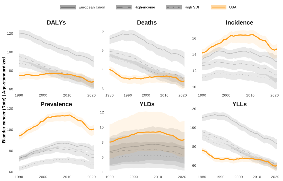
Figure 1: Age-standardized bladder cancer burden rates (per 100,000; both sexes) in the U.S. compared with the high-income and high-SDI aggregates (which include the U.S.) and the European Union. Incidence, prevalence, YLDs and DALYs are available from 1990, deaths and YLLs from 1980.

Abbreviations: DALYs: disability-adjusted life years; YLDs: years lived with disability; YLLs: years of life lost; EU: European Union; SDI: Socio-Demographic Index.

In [16]:

measure_order <- c("Incidence", "Prevalence", "Deaths", "YLDs", "YLLs", "DALYs")
measure_disp <- c(Incidence = "Incidence", Prevalence = "Prevalence", Deaths = "Mortality", 
                  YLDs = "YLDs", YLLs = "YLLs", DALYs = "DALYs")

t1_a <- chg90 %>% filter(sex_id == 3, location_id %in% comp_ids)
t1_b <- chg10 %>% filter(sex_id == 3, location_id %in% comp_ids)

t1 <- 
  t1_a %>% 
  mutate(
    measure_name, location_id,
    r1990 = fmt_ui(val_start, lower_start, upper_start),
    r2021 = fmt_ui(val_end, lower_end, upper_end),
    c9021 = fmt_pct(pct, pct_lower, pct_upper)
  ) %>% 
  left_join(
    t1_b %>% mutate(measure_name, location_id, c1021 = fmt_pct(pct, pct_lower, pct_upper)),
    by = c("measure_name", "location_id")
  ) %>% 
  mutate(
    Measure = factor(unname(measure_disp[measure_name]), levels = unname(measure_disp[measure_order])),
    Region = unname(region_labels[as.character(location_id)]),
    ord = match(location_id, comp_ids)
  ) %>% 
  arrange(Measure, ord) %>% 
  mutate(
    Measure = as.character(Measure), Region, 
    `1990` = r1990, `2021` = r2021, 
    `% change 1990–2021` = c9021, `% change 2010–2021` = c1021
  )

# TRUE when both UI bounds share the same sign (UI excludes zero)
sig_pos <- function(lo, hi) !is.na(lo) & !is.na(hi) & lo > 0 & hi > 0
sig_neg <- function(lo, hi) !is.na(lo) & !is.na(hi) & lo < 0 & hi < 0

# 1990–2021 uses the .x columns, 2010–2021 uses the .y columns
t1 <- t1 %>% 
  mutate(
    pos_9021 = sig_pos(pct_lower.x, pct_upper.x),
    neg_9021 = sig_neg(pct_lower.x, pct_upper.x),
    pos_1021 = sig_pos(pct_lower.y, pct_upper.y),
    neg_1021 = sig_neg(pct_lower.y, pct_upper.y)
  )

ft <- flextable(
  t1,
  col_keys = c('Measure', 'Region', '1990', '2021', '% change 1990–2021', '% change 2010–2021')
) %>% 
  merge_v(j = "Measure") %>% 
  valign(j = "Measure", valign = "top") %>% 
  fontsize(size = 8, part = "all")

ft <- ft %>% 
  color(i = which(t1$pos_9021), j = "% change 1990–2021", color = "darkred") %>%
  color(i = which(t1$neg_9021), j = "% change 1990–2021", color = "darkgreen") %>%
  color(i = which(t1$pos_1021), j = "% change 2010–2021", color = "darkred") %>%
  color(i = which(t1$neg_1021), j = "% change 2010–2021", color = "darkgreen") %>%
  autofit() %>% 
  fit_to_width(max_width = 6.5)

ft %>% flextable::save_as_docx(path = "output/tables/table1.docx")

ft

In [17]:

Table 1: Age-standardized rates (per 100,000; both sexes) and percent change, U.S. and comparator regions. Values are point estimate [95% UI]. Percent-change UIs are approximate (see Methods, Section 3.3.2); the U.S. is part of the high-income and high-SDI aggregates. Changes with both UIs on positive or negative are colored in red and green, respectively.

Measure	Region	1990	2021	% change 1990–2021	% change 2010–2021
Incidence	United States	14.2 [13.5, 14.7]	14.7 [13.6, 15.4]	+3.6% [−3.7%, +11.4%]	−10.5% [−17.4%, −3.1%]
	European Union	13.4 [12.8, 13.8]	13.1 [12.1, 13.9]	−2.3% [−9.6%, +5.7%]	−8.7% [−15.9%, −0.9%]
	High-income	12.6 [12.0, 13.0]	11.5 [10.6, 12.0]	−9.1% [−15.7%, −1.9%]	−10.1% [−17.1%, −2.4%]
	High SDI	11.2 [10.7, 11.6]	10.6 [9.8, 11.1]	−5.3% [−12.2%, +2.1%]	−7.7% [−14.9%, 0.0%]
Prevalence	United States	94.0 [90.6, 96.8]	100.6 [95.0, 104.6]	+7.0% [+1.0%, +13.5%]	−11.4% [−16.8%, −5.7%]
	European Union	72.2 [69.5, 74.5]	80.6 [75.8, 85.2]	+11.6% [+4.3%, +19.5%]	−7.6% [−13.7%, −1.1%]
	High-income	73.0 [70.5, 75.2]	73.8 [69.1, 77.0]	+1.1% [−5.0%, +7.6%]	−9.4% [−15.1%, −3.3%]
	High SDI	63.6 [61.2, 65.4]	66.8 [62.8, 69.6]	+5.1% [−1.1%, +11.6%]	−7.1% [−12.7%, −1.2%]
Mortality	United States	3.5 [3.3, 3.7]	3.4 [3.0, 3.6]	−3.0% [−12.8%, +7.9%]	−6.3% [−16.6%, +5.2%]
	European Union	5.8 [5.5, 6.0]	4.6 [4.1, 4.9]	−21.2% [−28.4%, −13.2%]	−8.9% [−17.9%, +1.1%]
	High-income	4.7 [4.4, 4.9]	3.5 [3.1, 3.7]	−25.7% [−33.0%, −17.8%]	−10.2% [−19.8%, +0.6%]
	High SDI	4.4 [4.1, 4.5]	3.4 [3.0, 3.6]	−21.9% [−29.5%, −13.6%]	−8.0% [−17.5%, +2.7%]
YLDs	United States	8.0 [5.8, 10.4]	8.4 [6.1, 10.8]	+4.1% [−30.6%, +56.4%]	−11.0% [−40.4%, +33.0%]
	European Union	6.7 [4.9, 8.7]	7.1 [5.2, 9.4]	+6.2% [−29.7%, +60.3%]	−7.7% [−39.0%, +39.7%]
	High-income	6.6 [4.8, 8.5]	6.4 [4.6, 8.2]	−3.4% [−35.5%, +44.7%]	−9.5% [−39.6%, +35.7%]
	High SDI	5.8 [4.2, 7.5]	5.8 [4.3, 7.5]	+0.1% [−33.1%, +49.7%]	−7.2% [−37.8%, +38.4%]
YLLs	United States	66.6 [63.2, 68.8]	59.8 [55.1, 62.6]	−10.1% [−16.8%, −2.9%]	−9.9% [−17.1%, −2.1%]
	European Union	112.7 [108.1, 115.8]	82.9 [76.9, 87.8]	−26.4% [−31.7%, −20.7%]	−11.8% [−18.4%, −4.6%]
	High-income	88.5 [84.4, 91.1]	60.4 [55.6, 63.6]	−31.7% [−36.7%, −26.2%]	−13.5% [−20.4%, −5.9%]
	High SDI	82.1 [78.3, 84.6]	59.3 [54.7, 62.4]	−27.8% [−33.1%, −22.1%]	−11.4% [−18.3%, −4.0%]
DALYs	United States	74.6 [70.4, 78.1]	68.1 [62.7, 72.5]	−8.6% [−16.4%, −0.1%]	−10.1% [−18.1%, −1.2%]
	European Union	119.4 [114.7, 123.4]	90.1 [83.3, 96.0]	−24.6% [−30.4%, −18.3%]	−11.5% [−18.7%, −3.6%]
	High-income	95.1 [90.8, 98.6]	66.8 [61.6, 70.9]	−29.7% [−35.2%, −23.8%]	−13.1% [−20.4%, −5.1%]
	High SDI	87.9 [84.0, 91.2]	65.1 [60.1, 68.7]	−26.0% [−31.6%, −20.0%]	−11.1% [−18.3%, −3.2%]

Abbreviations: UI, uncertainty interval; SDI, Socio-Demographic Index; YLDs, years lived with disability; YLLs, years of life lost; DALYs, disability-adjusted life years.

For both sexes combined, the percent change in the ASR of mortality between 1990 and 2021 was, by region (percent change [approximate 95% UI]): United States −3.0% [−12.8%, +7.9%]; European Union −21.2% [−28.4%, −13.2%]; High-income −25.7% [−33.0%, −17.8%]; High SDI −21.9% [−29.5%, −13.6%]. For DALYs it was: United States −8.6% [−16.4%, −0.1%]; European Union −24.6% [−30.4%, −18.3%]; High-income −29.7% [−35.2%, −23.8%]; High SDI −26.0% [−31.6%, −20.0%]. For incidence it was: United States +3.6% [−3.7%, +11.4%]; European Union −2.3% [−9.6%, +5.7%]; High-income −9.1% [−15.7%, −1.9%]; High SDI −5.3% [−12.2%, +2.1%]; and between 2010 and 2021: United States −10.5% [−17.4%, −3.1%]; European Union −8.7% [−15.9%, −0.9%]; High-income −10.1% [−17.1%, −2.4%]; High SDI −7.7% [−14.9%, 0.0%]. Sex-specific values, and values for all other measures and for every jurisdiction, are in Supporting Info 1 and, as a graphical table, Supporting Info 3. Because the percent-change intervals are approximate and no trend model was fitted, we describe these as differences between years, not as tests of trend. Because the high-income and high-SDI aggregates contain the U.S., differences between the U.S. and these aggregates are attenuated by construction.

4.2 Age and sex patterns in the U.S.

As illustrated in Figure 2, in 2021 the male rate exceeded the female rate in 84 of 96 age-group–by–measure combinations. The highest 2021 age-specific rates (per 100,000) were: DALYs, women (80+ years): 462.3 [354.7, 521.8]; men (80+ years): 1,617.1 [1,365.6, 1,752.9]. mortality, women (80+ years): 42.1 [31.9, 47.5]; men (80+ years): 142.2 [118.3, 154.5]. incidence, women (80+ years): 84.1 [63.8, 94.5]; men (80+ years): 309.3 [258.4, 335.0]. prevalence, women (75-79 years): 411.0 [358.2, 441.0]; men (75-79 years): 1,481.3 [1,366.4, 1,568.7]. YLDs, women (80+ years): 37.8 [26.7, 48.8]; men (80+ years): 136.1 [99.5, 174.7]. YLLs, women (80+ years): 424.6 [323.9, 477.4]; men (80+ years): 1,481.0 [1,241.4, 1,606.1].

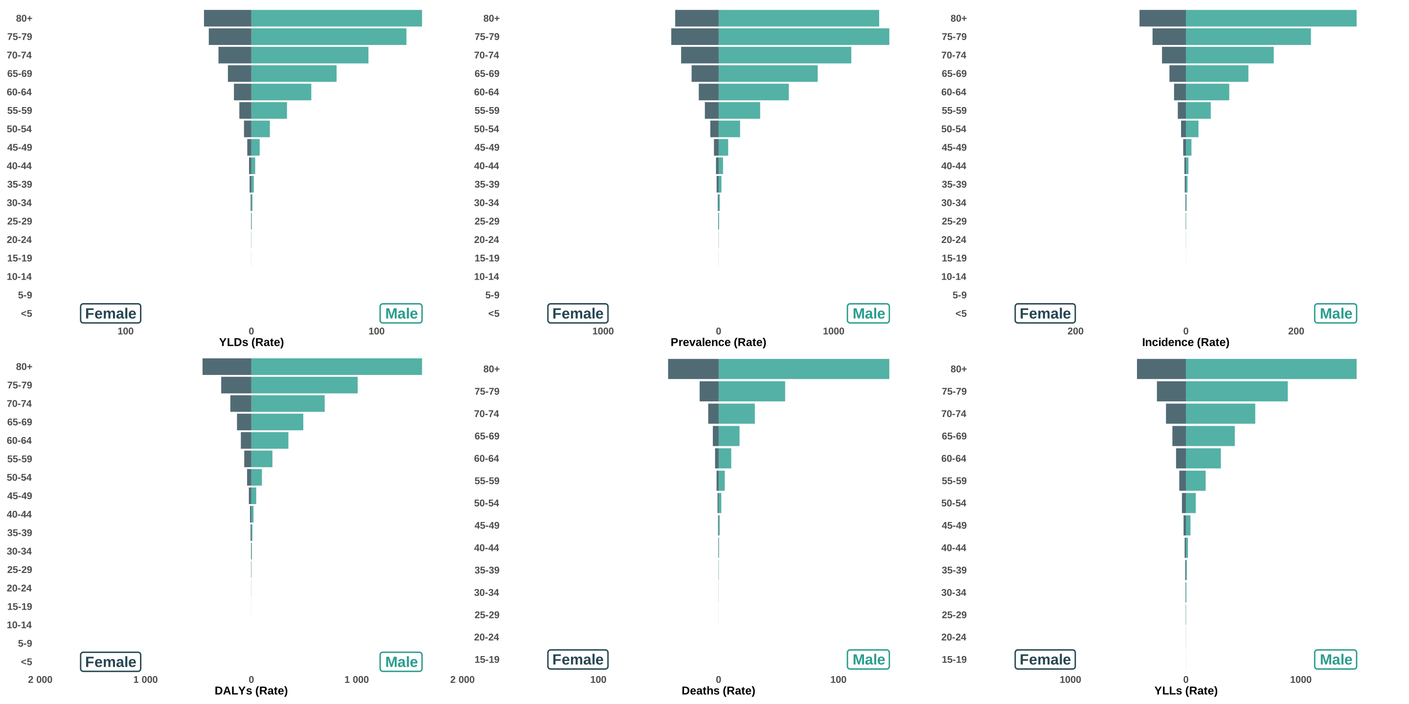
Figure 2: Population pyramids showing age- and sex-specific bladder cancer burden rates (per 100,000) in the U.S., 2021.

Abbreviations: DALYs: disability-adjusted life years; YLDs: years lived with disability; YLLs: years of life lost.

State-level population pyramids for 2021 are provided in Supporting Info 4, and animated pyramids showing change by year for each state and the U.S. in Supporting Info 5. Figure 3 displays age-specific rates in 1990, 2000, 2010 and 2021 by sex. It is a descriptive age-by-period display; no age–period–cohort model was fitted. Corresponding plots for each state are in Supporting Info 6.

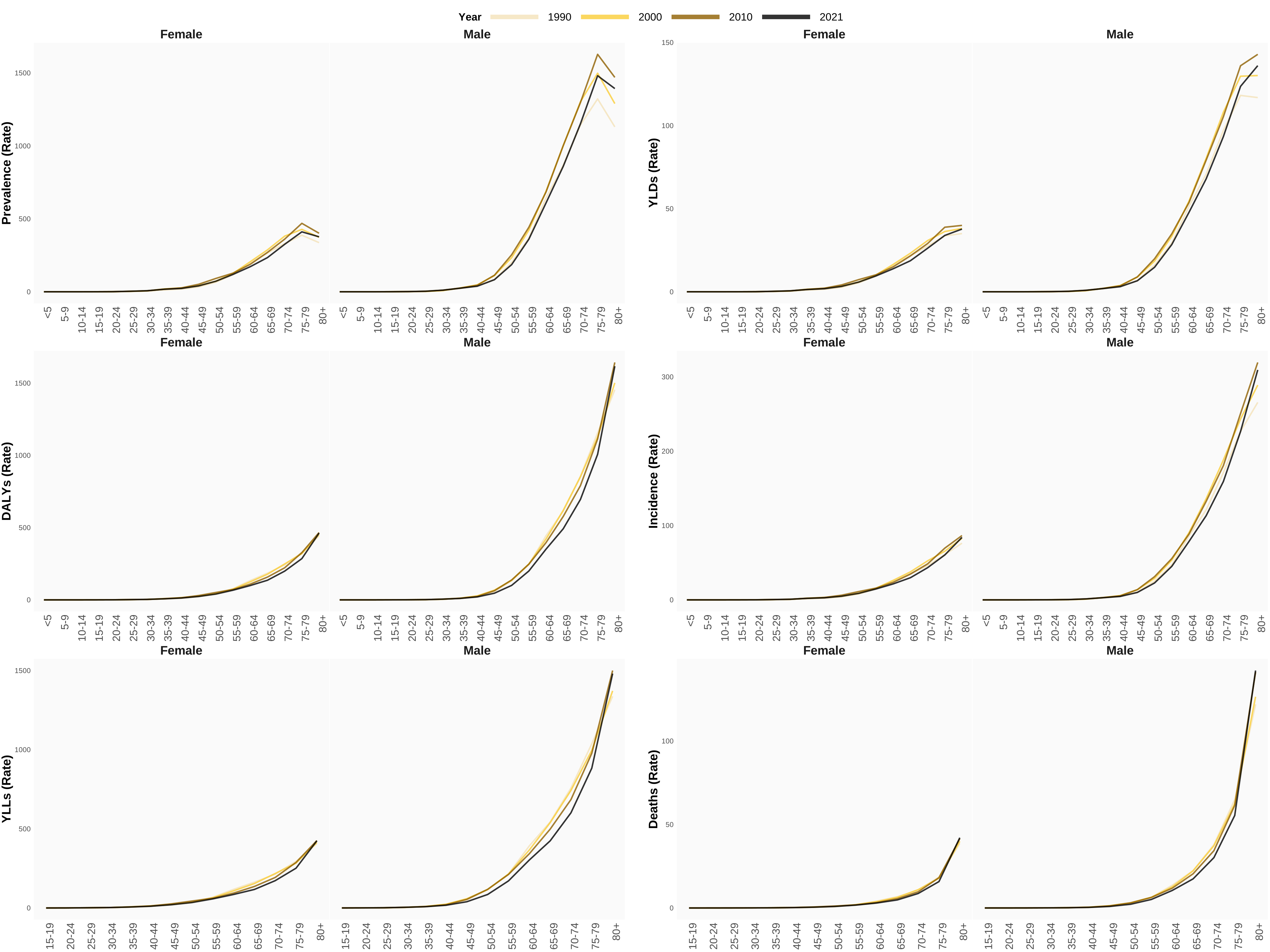
Figure 3: Age-specific bladder cancer burden rates (per 100,000) by sex in the U.S. in 1990, 2000, 2010 and 2021 (descriptive; no age–period–cohort model fitted).

Abbreviations: DALYs: disability-adjusted life years; YLDs: years lived with disability; YLLs: years of life lost.

Absolute case and death counts were not part of the extracted dataset; we therefore cannot report changes in the number of cases.

4.3 Bladder cancer burden across U.S. states

State-specific, sex-stratified temporal trends in age-standardized incidence rates are displayed in Figure 4; geofaceted plots for the other five measures are provided in Supporting Info 7.

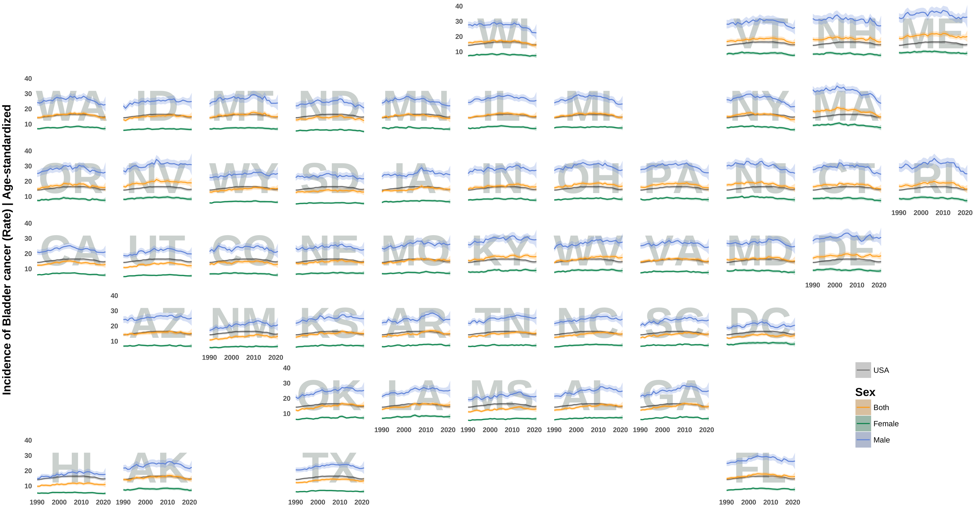
Figure 4: State-level historical trends in age-standardized bladder cancer *incidence* rates (per 100,000), U.S., stratified by sex. States are arranged to approximate their geographic location; the grey band is the U.S. (both sexes).

Abbreviations: Alabama: AL; Alaska: AK; Arizona: AZ; Arkansas: AR; California: CA; Colorado: CO; Connecticut: CT; Delaware: DE; District of Columbia: DC; Florida: FL; Georgia: GA; Hawaii: HI; Idaho: ID; Illinois: IL; Indiana: IN; Iowa: IA; Kansas: KS; Kentucky: KY; Louisiana: LA; Maine: ME; Maryland: MD; Massachusetts: MA; Michigan: MI; Minnesota: MN; Mississippi: MS; Missouri: MO; Montana: MT; Nebraska: NE; Nevada: NV; New Hampshire: NH; New Jersey: NJ; New Mexico: NM; New York: NY; North Carolina: NC; North Dakota: ND; Ohio: OH; Oklahoma: OK; Oregon: OR; Pennsylvania: PA; Rhode Island: RI; South Carolina: SC; South Dakota: SD; Tennessee: TN; Texas: TX; Utah: UT; Vermont: VT; Virginia: VA; Washington: WA; West Virginia: WV; Wisconsin: WI; Wyoming: WY.

Table 2 lists the 2021 age-standardized incidence and mortality rates (both sexes), the rank of each jurisdiction by point estimate (1 = highest), and the percent change since 1990. By point estimate, the highest 2021 incidence ASRs (both sexes, per 100,000) were in Maine (19.9), Nevada (18.9), Delaware (18.6), Kentucky (18.0), and West Virginia (17.5) and the lowest in Hawaii (11.0), Utah (12.0), North Dakota (12.3), California (12.8), and South Dakota (12.9); the highest 2021 mortality ASRs were in Maine (4.5), Nevada (4.3), Kentucky (4.2), Delaware (4.2), and West Virginia (4.1) and the lowest in Hawaii (2.3), North Dakota (2.8), California (2.9), New York (2.9), and Utah (3.0). These are rankings of point estimates; the published 95% UIs of the 2021 ASR overlapped for 97% of all pairs of jurisdictions for incidence and 95% for mortality (Table 2), so the ranking itself is uncertain. Between 1990 and 2021, the largest point-estimate decreases in incidence ASR were in Massachusetts (−21.2%), New York (−14.1%), New Jersey (−11.9%), Rhode Island (−11.3%), and Wisconsin (−9.9%), and the smallest decreases or largest increases in West Virginia (+25.4%), Louisiana (+24.6%), Oklahoma (+24.5%), Alabama (+23.5%), and New Mexico (+22.4%). The approximate UI of the 1990–2021 percent change in incidence lay entirely below zero in 1 of 51 jurisdictions, entirely above zero in 6, and included zero in 44; for mortality the corresponding numbers were 2, 1 and 48. Rates by sex for all six measures are in Supporting Info 1.

In [18]:

state_chg <- chg90 %>% filter(location_id %in% c(stateids, us_id), sex_id == 3)

state_block <- function(measure, prefix) {
  state_chg %>%
    filter(measure_name == measure) %>%
    mutate(
      val_for_rank = if_else(location_id == us_id, NA_real_, val_end),
      rank = min_rank(desc(val_for_rank))
    ) %>%
    mutate(
      location_id,
      "{prefix}_rate" := fmt_ui(val_end, lower_end, upper_end),
      "{prefix}_rank" := if_else(is.na(rank), "–", as.character(rank)),
      "{prefix}_chg"  := fmt_pct(pct, pct_lower, pct_upper)
    )
}

state_table <- 
  state_chg %>% 
  filter(measure_name == "Incidence") %>% 
  select(location_id, Jurisdiction = location_name) %>% 
  left_join(state_block("Incidence", "inc"), by = "location_id") %>% 
  left_join(state_block("Deaths", "mor"), by = "location_id") %>% 
  arrange(location_id != us_id, Jurisdiction) %>% 
  select(-location_id)

f2 <- 
  flextable(
    state_table, 
    col_keys = c("Jurisdiction", "inc_rate", "inc_rank", "inc_chg", "mor_rate", "mor_rank", "mor_chg")
  ) %>% 
  set_header_labels(
    inc_rate = "2021 rate", inc_rank = "Rank", inc_chg = "% change 1990–2021",
    mor_rate = "2021 rate", mor_rank = "Rank", mor_chg = "% change 1990–2021"
  ) %>% 
  add_header_row(values = c("", "Incidence", "Mortality"), colwidths = c(1, 3, 3)) %>% 
  fontsize(size = 7, part = "all") %>% 
  color(~ ((sign(pct_lower.x) == sign(pct_upper.x)) & sign(pct_lower.x) > 0), ~ inc_chg, color = "darkred") %>%
  color(~ ((sign(pct_lower.x) == sign(pct_upper.x)) & sign(pct_lower.x) < 0), ~ inc_chg, color = "darkgreen") %>%
  color(~ ((sign(pct_lower.y) == sign(pct_upper.y)) & sign(pct_lower.y) > 0), ~ mor_chg, color = "darkred") %>%
  color(~ ((sign(pct_lower.y) == sign(pct_upper.y)) & sign(pct_lower.y) < 0), ~ mor_chg, color = "darkgreen") %>%
  autofit() %>% 
  fit_to_width(max_width = 6.5)

f2 %>% flextable::save_as_docx(path = "output/tables/table2.docx")

f2

In [19]:

Table 2: Age-standardized incidence and mortality rates (per 100,000; both sexes), 2021, rank among the 50 states and DC by point estimate (1 = highest), and percent change 1990–2021, with 95% UI (percent-change UIs approximate). Changes with both UIs on positive or negative are colored in red and green, respectively.

	Incidence			Mortality
Jurisdiction	2021 rate	Rank	% change 1990–2021	2021 rate	Rank	% change 1990–2021
United States of America	14.7 [13.6, 15.4]	–	+3.6% [−3.7%, +11.4%]	3.4 [3.0, 3.6]	–	−3.0% [−12.8%, +7.9%]
Alabama	15.0 [12.6, 17.8]	25	+23.5% [+2.2%, +49.2%]	3.8 [3.2, 4.4]	9	+15.5% [−3.8%, +38.8%]
Alaska	14.6 [12.5, 16.9]	34	+2.8% [−13.3%, +21.9%]	3.3 [2.8, 3.8]	42	−13.6% [−28.1%, +3.9%]
Arizona	15.3 [12.8, 18.3]	19	+6.6% [−12.3%, +29.5%]	3.4 [2.8, 4.0]	34	−2.7% [−19.8%, +18.0%]
Arkansas	15.0 [12.5, 17.7]	26	+15.7% [−4.1%, +39.6%]	3.7 [3.1, 4.3]	13	+7.7% [−10.6%, +29.8%]
California	12.8 [10.7, 14.9]	48	+3.6% [−13.5%, +24.1%]	2.9 [2.4, 3.4]	49	−8.8% [−23.7%, +8.9%]
Colorado	13.0 [10.5, 15.6]	44	+1.4% [−18.1%, +25.6%]	3.0 [2.4, 3.6]	45	−1.0% [−20.8%, +23.7%]
Connecticut	14.9 [12.1, 17.8]	28	−8.3% [−25.5%, +12.9%]	3.5 [2.8, 4.1]	29	−9.5% [−26.3%, +11.2%]
Delaware	18.6 [15.8, 21.5]	3	+9.5% [−7.5%, +29.6%]	4.2 [3.6, 4.9]	4	−2.8% [−18.1%, +15.3%]
District of Columbia	13.7 [11.3, 16.4]	40	+11.5% [−8.4%, +35.7%]	3.3 [2.7, 3.9]	41	−25.1% [−38.1%, −9.4%]
Florida	16.1 [13.3, 19.0]	9	+9.1% [−9.9%, +32.1%]	3.5 [2.9, 4.2]	20	+0.2% [−17.7%, +21.9%]
Georgia	14.7 [12.2, 17.6]	31	+21.0% [−0.3%, +46.9%]	3.6 [3.0, 4.2]	18	+7.2% [−10.8%, +29.0%]
Hawaii	11.0 [9.1, 13.2]	51	+12.2% [−8.8%, +38.1%]	2.3 [1.9, 2.8]	51	−2.9% [−22.0%, +20.8%]
Idaho	15.0 [12.3, 17.8]	24	+16.1% [−5.0%, +41.9%]	3.7 [3.0, 4.3]	15	+13.7% [−6.8%, +38.8%]
Illinois	15.3 [12.8, 18.1]	21	+7.3% [−10.9%, +29.3%]	3.5 [2.9, 4.2]	19	−1.9% [−18.8%, +18.5%]
Indiana	16.3 [13.5, 19.3]	8	+10.9% [−8.6%, +34.5%]	3.9 [3.2, 4.6]	7	+9.8% [−9.3%, +32.9%]
Iowa	14.5 [12.1, 17.4]	36	+11.1% [−8.9%, +35.5%]	3.3 [2.8, 4.0]	37	+10.7% [−8.1%, +33.4%]
Kansas	15.0 [12.4, 18.1]	23	+19.6% [−2.6%, +46.9%]	3.4 [2.9, 4.0]	33	+20.0% [−0.9%, +45.2%]
Kentucky	18.0 [15.1, 21.4]	4	+16.3% [−3.5%, +40.1%]	4.2 [3.5, 5.0]	3	+15.5% [−4.0%, +39.0%]
Louisiana	15.8 [13.3, 18.6]	12	+24.6% [+4.0%, +49.2%]	3.8 [3.2, 4.4]	10	+12.7% [−5.3%, +34.1%]
Maine	19.9 [16.5, 24.0]	1	+5.8% [−13.7%, +29.9%]	4.5 [3.8, 5.4]	1	+3.6% [−14.7%, +25.9%]
Maryland	15.3 [12.6, 18.1]	20	−4.9% [−21.8%, +15.7%]	3.5 [2.9, 4.1]	23	−15.3% [−30.3%, +2.8%]
Massachusetts	14.6 [12.0, 17.5]	33	−21.2% [−35.7%, −3.4%]	3.4 [2.8, 4.1]	31	−15.2% [−30.2%, +3.0%]
Michigan	14.5 [12.3, 17.1]	35	+1.6% [−15.0%, +21.6%]	3.5 [2.9, 4.0]	27	−6.1% [−21.3%, +12.0%]
Minnesota	13.7 [11.2, 16.4]	41	−4.4% [−22.0%, +17.1%]	3.3 [2.6, 3.8]	40	+4.2% [−15.0%, +27.7%]
Mississippi	13.0 [11.0, 15.4]	45	+16.9% [−2.7%, +40.3%]	3.4 [2.9, 3.9]	36	+8.6% [−8.8%, +29.3%]
Missouri	15.7 [13.1, 18.6]	14	+14.9% [−4.9%, +38.9%]	3.6 [3.1, 4.2]	17	+8.2% [−8.9%, +28.6%]
Montana	14.9 [12.3, 17.6]	27	+6.7% [−12.2%, +29.6%]	3.5 [2.9, 4.2]	24	+0.5% [−17.6%, +22.4%]
Nebraska	14.2 [11.8, 16.8]	39	+3.4% [−15.0%, +25.9%]	3.3 [2.7, 3.9]	39	+6.0% [−13.4%, +29.9%]
Nevada	18.9 [15.4, 22.5]	2	+14.0% [−7.0%, +39.8%]	4.3 [3.5, 5.0]	2	+1.2% [−17.1%, +23.4%]
New Hampshire	16.5 [13.4, 19.8]	7	−9.1% [−26.3%, +12.1%]	3.9 [3.2, 4.6]	8	−6.8% [−24.4%, +15.1%]
New Jersey	15.4 [12.7, 18.4]	15	−11.9% [−27.8%, +7.5%]	3.5 [2.9, 4.2]	26	−16.6% [−31.5%, +1.6%]
New Mexico	13.2 [11.0, 15.6]	43	+22.4% [+0.8%, +48.6%]	3.0 [2.5, 3.6]	44	+2.7% [−15.8%, +25.4%]
New York	13.0 [10.6, 15.4]	46	−14.1% [−29.5%, +4.7%]	2.9 [2.4, 3.5]	48	−24.5% [−38.4%, −7.5%]
North Carolina	14.8 [12.4, 17.6]	30	+19.5% [−0.9%, +44.2%]	3.5 [2.9, 4.1]	28	+8.7% [−10.2%, +31.7%]
North Dakota	12.3 [10.3, 14.3]	49	−3.4% [−20.0%, +16.6%]	2.8 [2.3, 3.3]	50	−5.0% [−21.3%, +14.8%]
Ohio	16.8 [13.9, 19.8]	6	+7.9% [−10.7%, +30.4%]	4.0 [3.4, 4.7]	6	+6.0% [−11.4%, +26.8%]
Oklahoma	15.4 [12.9, 18.2]	16	+24.5% [+3.2%, +50.2%]	3.7 [3.1, 4.3]	11	+23.7% [+3.1%, +48.4%]
Oregon	16.0 [13.2, 19.3]	11	+7.7% [−12.3%, +32.2%]	3.5 [3.0, 4.2]	22	+1.5% [−16.9%, +24.1%]
Pennsylvania	15.7 [13.0, 18.7]	13	−2.6% [−20.0%, +18.5%]	3.7 [3.0, 4.4]	14	−6.0% [−23.0%, +14.9%]
Rhode Island	14.9 [12.2, 17.6]	29	−11.3% [−27.6%, +8.7%]	3.5 [2.9, 4.2]	25	−11.5% [−27.2%, +7.6%]
South Carolina	14.7 [12.1, 17.1]	32	+20.8% [+0.5%, +45.2%]	3.5 [3.0, 4.1]	21	+4.2% [−12.5%, +24.0%]
South Dakota	12.9 [10.9, 15.2]	47	+2.8% [−14.7%, +24.0%]	3.0 [2.5, 3.6]	46	−1.2% [−18.9%, +20.4%]
Tennessee	15.3 [12.8, 18.1]	18	+19.6% [−0.7%, +44.1%]	3.7 [3.1, 4.2]	16	+11.0% [−7.2%, +32.6%]
Texas	13.3 [11.3, 15.5]	42	+9.7% [−7.4%, +29.9%]	3.1 [2.6, 3.6]	43	+0.8% [−15.4%, +20.1%]
Utah	12.0 [10.0, 14.3]	50	+11.2% [−8.5%, +35.3%]	3.0 [2.5, 3.5]	47	+6.2% [−12.7%, +29.3%]
Vermont	16.1 [13.6, 18.6]	10	−3.1% [−18.9%, +15.7%]	3.7 [3.0, 4.3]	12	−9.8% [−25.3%, +9.0%]
Virginia	15.1 [12.5, 18.0]	22	+3.8% [−14.5%, +26.1%]	3.4 [2.8, 4.1]	32	−3.9% [−21.1%, +17.1%]
Washington	14.3 [11.8, 16.9]	37	−0.4% [−17.9%, +20.9%]	3.3 [2.7, 3.9]	38	−1.7% [−19.1%, +19.3%]
West Virginia	17.5 [14.7, 20.3]	5	+25.4% [+5.0%, +49.7%]	4.1 [3.5, 4.8]	5	+15.3% [−3.1%, +37.0%]
Wisconsin	14.2 [11.8, 17.2]	38	−9.9% [−26.3%, +10.2%]	3.4 [2.8, 4.1]	35	−6.5% [−23.9%, +14.8%]
Wyoming	15.4 [13.0, 17.7]	17	+18.7% [−0.1%, +41.1%]	3.5 [2.9, 3.9]	30	+5.9% [−10.9%, +25.9%]

Figure 5 displays male-to-female rate ratios of ASRs in 2021 for each jurisdiction and measure. Because incidence is derived from mortality and prevalence and YLDs are derived from incidence and survival in the GBD cancer models (20), the six ratios are strongly related by construction and are not independent evidence; we therefore describe incidence and mortality. Across the 50 states and DC, male:female incidence rate ratios ranged from District of Columbia, 2.5 [1.8, 3.4] (lowest point estimate) to North Dakota, 4.1 [3.1, 5.4] (highest point estimate), and mortality ratios from District of Columbia, 2.4 [1.8, 3.2] to South Dakota, 4.2 [3.2, 5.6] (ratio [approximate 95% UI]). The approximate UIs of the lowest and highest jurisdictions overlapped for incidence and overlapped for mortality. These UIs assume independence between the male and female estimates (Section 3.3.2) and must not be read as a test of a difference between jurisdictions. For the U.S. overall, the 2021 male:female incidence ratio was 3.4 [3.1, 3.8]. All ratios are in Supporting Info 2.

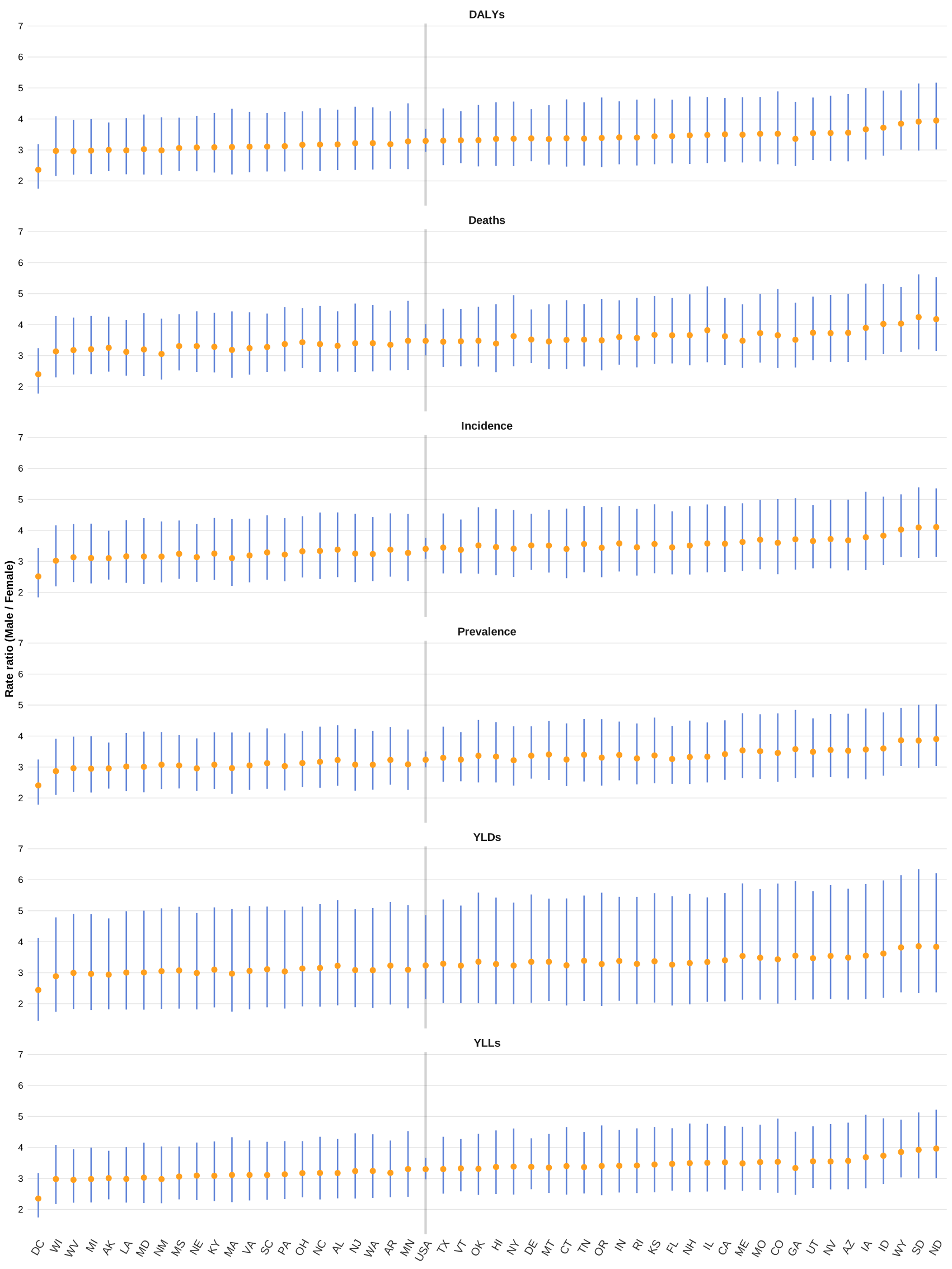
Figure 5: State-level male:female ratio of age-standardized rates, 2021, by measure (point estimates with approximate 95% UIs that assume independence of the male and female estimates; see Methods).

Abbreviations: Alabama: AL; Alaska: AK; Arizona: AZ; Arkansas: AR; California: CA; Colorado: CO; Connecticut: CT; Delaware: DE; District of Columbia: DC; Florida: FL; Georgia: GA; Hawaii: HI; Idaho: ID; Illinois: IL; Indiana: IN; Iowa: IA; Kansas: KS; Kentucky: KY; Louisiana: LA; Maine: ME; Maryland: MD; Massachusetts: MA; Michigan: MI; Minnesota: MN; Mississippi: MS; Missouri: MO; Montana: MT; Nebraska: NE; Nevada: NV; New Hampshire: NH; New Jersey: NJ; New Mexico: NM; New York: NY; North Carolina: NC; North Dakota: ND; Ohio: OH; Oklahoma: OK; Oregon: OR; Pennsylvania: PA; Rhode Island: RI; South Carolina: SC; South Dakota: SD; Tennessee: TN; Texas: TX; Utah: UT; Vermont: VT; Virginia: VA; Washington: WA; West Virginia: WV; Wisconsin: WI; Wyoming: WY; DALYs: disability-adjusted life years; YLDs: years lived with disability; YLLs: years of life lost.

In [20]:

# Saves the sex-ratio figure (fig_H.svg) from the corrected ratios
invisible(gender_discrep_plot(discrep_data))

Warning: Using `size` aesthetic for lines was deprecated in ggplot2 3.4.0.
ℹ Please use `linewidth` instead.

Warning: The `size` argument of `element_line()` is deprecated as of ggplot2 3.4.0.
ℹ Please use the `linewidth` argument instead.

Bump plots comparing the U.S., all jurisdictions and the comparator regions across measures in 1990, 2000, 2010 and 2021 are in Supporting Info 8.

5 Discussion

5.1 Principal findings

In this descriptive analysis of GBD 2021 estimates, the U.S. age-standardized incidence rate of BC in 2021 was 14.7 [13.6, 15.4] per 100,000 and the age-standardized mortality rate 3.4 [3.0, 3.6] per 100,000 (both sexes). The incidence ASR peaked in 2011; between 2010 and 2021 it changed by −10.5% [−17.4%, −3.1%], and between 1990 and 2021 by +3.6% [−3.7%, +11.4%]. The mortality ASR changed by −3.0% [−12.8%, +7.9%] between 1990 and 2021 and by −6.3% [−16.6%, +5.2%] between 2010 and 2021 (percent change [approximate 95% UI]). We did not fit a trend model, so these are differences between years and not statements about the statistical significance of a trend. Across jurisdictions, estimated changes since 1990 varied (Table 2); for 44 of 51 jurisdictions the approximate UI of the incidence change included zero. All of these results are modelled estimates, and no exposure, policy or health-system variable was analysed; explanations offered below are hypotheses drawn from the literature, not findings of this study.

5.2 Comparison with other regions

The numbers of years in which the U.S. point estimate of incidence exceeded that of each comparator are given in Section 4.1. The high-income and high-SDI aggregates contain the U.S., so those contrasts are attenuated by construction and are not independent country-to-country comparisons; the European Union is the only comparator that excludes the U.S. A higher estimated incidence in the U.S. may partly reflect more intensive diagnostic activity (cystoscopy, imaging, and evaluation of hematuria) and case ascertainment (27–29), which raises recorded incidence without necessarily changing mortality, and/or differences in underlying risk, such as smoking history. This study cannot separate these possibilities, which are not mutually exclusive. Registry-based age-adjusted rates (for example, the SEER rate of about 18 per 100,000 for 2018–2022 (2)) are not directly comparable with GBD ASRs, which use a different standard population and are modelled.

5.3 Age

Age-standardized and age-specific rates are by design unaffected by population ageing; the rates reported here therefore cannot be attributed to population ageing. Ageing influences the number of cases: the U.S. population aged 65 years and older increased by 38.6% between 2010 and 2020 (30). Absolute case and death counts were not part of the extracted dataset; we therefore cannot report changes in the number of cases. The age groups with the highest age-specific rates are reported in Section 4.2; a rise in BC burden with age is in line with prior literature (4). An earlier analysis reported that the oldest adults, especially men aged 85 years and older, had not shared in the improvements in cancer mortality seen in younger seniors (31). We did not examine whether differences between states in age-specific rates reflect true differences, and we do not interpret them.

5.4 Sex differences

Male rates exceeded female rates in 84 of 96 age-group–by–measure combinations in 2021 (Section 4.2). The 2021 U.S. male:female incidence ratio was 3.4 [3.1, 3.8], and prior studies consistently report three- to four-fold higher incidence in men (3). For mortality, the 1990–2021 percent change was −6.7% [−15.3%, +2.8%] in men and −10.5% [−23.0%, +4.0%] in women. State-level ratios varied, with extremes of District of Columbia, 2.5 [1.8, 3.4] and North Dakota, 4.1 [3.1, 5.4] for incidence, but the approximate UIs are wide, assume independence of the male and female estimates, and the ratios are partly related across measures by construction (Section 3.1). GBD estimates contain no information on stage at diagnosis, treatment or survival. Studies outside GBD report that women more often present with advanced disease and have poorer survival (16,32,33), and that hematuria in women is more often attributed to urinary tract infection or gynecologic conditions (32,34). Differences in immune surveillance, hormonal milieu and genetic or epigenetic alterations have also been proposed (35). These are hypotheses that this analysis can neither support nor refute.

5.5 Geographic variation

By point estimate, the highest 2021 incidence ASRs were in Maine (19.9), Nevada (18.9), Delaware (18.6), Kentucky (18.0), and West Virginia (17.5) and the lowest in Hawaii (11.0), Utah (12.0), North Dakota (12.3), California (12.8), and South Dakota (12.9); the highest mortality ASRs were in Maine (4.5), Nevada (4.3), Kentucky (4.2), Delaware (4.2), and West Virginia (4.1) and the lowest in Hawaii (2.3), North Dakota (2.8), California (2.9), New York (2.9), and Utah (3.0) (Table 2). Because the published UIs overlap for 97% (incidence) and 95% (mortality) of all pairs of jurisdictions, these rankings are uncertain, and our data do not establish that any particular jurisdiction differs from another. Earlier registry-based reports describe high incidence in northeastern states (11) and elevated mortality in parts of the South (14,36). Explanations that have been proposed, none of which we tested, include arsenic in private-well drinking water in New England (37,38), smoking-attributable burden (39), rurality (40,41), and reduced access to timely diagnosis and treatment (41,42); studies of other cancers, such as colorectal and cervical cancer, have linked longer travel distance to worse care (43). GBD state estimates are not stratified by race or ethnicity, so we cannot assess whether differences in population composition (for example, lower BC risk reported in Asian and Pacific Islander populations (44)) contribute to differences between states. DC is a federal district with a small, predominantly urban population, and is not directly comparable with the states.

5.6 Strengths and limitations

Strengths include the use of a single, internally consistent modelling framework across all states, six burden measures, and fully scripted, openly available, reproducible analyses. Limitations are as follows. First, GBD estimates are modelled; for many states the underlying data are sparse, and incidence, prevalence and YLDs depend on mortality-based modelling (20), so the six measures are not independent. Second, derived UIs (percent change and rate ratios) are approximations from published bounds that assume independence and log-symmetry, and the direction of any resulting bias is unknown (Section 3.3.2); draw-based UIs would be preferable. Third, the U.S. is part of two of the three comparator aggregates, and we did not include comparators that exclude the U.S. (for example, individual peer countries or Western Europe). Fourth, no trend model was fitted, and no exposure, insurance, socioeconomic or policy variable was analysed, so the study cannot address causes or policy effects. Fifth, the analysis is limited to rates; population ageing affects case counts, which are reported only where available. Sixth, estimates are not stratified by race or ethnicity. Seventh, GBD estimates are revised between rounds, and GBD 2023 estimates, including for cancer (19), are now available; values here may differ from GBD 2023, and repeating the scripted pipeline on the newer release is a natural next step. Finally, discrepancies with surveillance systems that report crude or differently standardized rates likely reflect methodological differences, including the choice of standard population.

6 Conclusions

GBD 2021 modelled estimates describe a male excess in BC burden in the U.S. in 2021, changes in age-standardized rates between 1990 and 2021 that are summarised in Table 1, and variation across states for which uncertainty is substantial. These findings are descriptive. Whether differences between states, sexes or regions are related to exposures, health-care access or policy cannot be determined from these data, and such questions require analyses that measure those factors directly. Since the submission of this manuscript, GBD 2023 data has been released. Should the data structure and dictionary remain the same as GBD 2021, all visualizations of this study are reproducible for GBD 2023 as well. We encourage future researchers to further the current study by forking our GitHub repository and applying its source code to GBD 2023.

Supporting Info

Supporting Info are provided as appendices to the manuscript and are also publicly accessible at the links below (repository: GitHub; archived version: 10.5281/zenodo.23814418).

Percent change (numeric table)
Percent change in age-standardized rates, with approximate 95% UIs, for 1990–2021 and 2010–2021 (all measures) and 1980–2021 (deaths and YLLs), for the U.S., all jurisdictions and comparator regions, by sex, together with the start- and end-year rates. CSV file.
Male:female rate ratios (2021, numeric table)
Male and female age-standardized rates and their ratio, with approximate 95% UIs (independence assumed), for every jurisdiction and measure. CSV file.
Percent change 1990–2021 (graphical table)
Percent change in age-standardized rates between 1990 and 2021, by sex, for the U.S., jurisdictions and comparator regions. Bars show the point estimate and lines the approximate 95% UI. Green, yellow and red indicate an interval entirely below zero, including zero, and entirely above zero, respectively (a description of the interval, not a significance test). Available from the project’s GitHub repository.
State-level population pyramids (2021)
Age- and sex-stratified bladder cancer burden for each jurisdiction in 2021, available from the project’s GitHub repository.
Animated population pyramids
Temporal change in age- and sex-stratified burden for each jurisdiction, available from the project’s GitHub repository.
Age-by-period plots
Line plots of age- and sex-specific rates in 1990, 2000, 2010 and 2021 for each jurisdiction (descriptive; no age–period–cohort model). The repository folder retains its original name, “APC plot 1”, available from the project’s GitHub repository.
Geographically faceted state-level plots (all six measures)
Available from the project’s GitHub repository.
Abbreviations: DALYs: disability-adjusted life years; YLDs: years lived with disability; YLLs: years of life lost; EU: European Union; SDI: Socio-Demographic Index; Alabama: AL; Alaska: AK; Arizona: AZ; Arkansas: AR; California: CA; Colorado: CO; Connecticut: CT; Delaware: DE; District of Columbia: DC; Florida: FL; Georgia: GA; Hawaii: HI; Idaho: ID; Illinois: IL; Indiana: IN; Iowa: IA; Kansas: KS; Kentucky: KY; Louisiana: LA; Maine: ME; Maryland: MD; Massachusetts: MA; Michigan: MI; Minnesota: MN; Mississippi: MS; Missouri: MO; Montana: MT; Nebraska: NE; Nevada: NV; New Hampshire: NH; New Jersey: NJ; New Mexico: NM; New York: NY; North Carolina: NC; North Dakota: ND; Ohio: OH; Oklahoma: OK; Oregon: OR; Pennsylvania: PA; Rhode Island: RI; South Carolina: SC; South Dakota: SD; Tennessee: TN; Texas: TX; Utah: UT; Vermont: VT; Virginia: VA; Washington: WA; West Virginia: WV; Wisconsin: WI; Wyoming: WY.
State ranking bump plots
Ranks of jurisdictions by point estimate in 1990, 2000, 2010 and 2021, available from the project’s GitHub repository.

Software
R version and attached package versions used for the analysis (table below).

In [21]:

sw <- sessionInfo()$otherPkgs
sw_tbl <-
  tibble(
    Package = c("R", names(sw)),
    Version = c(paste(R.version$major, R.version$minor, sep = "."), map_chr(sw, "Version"))
  )

flextable(sw_tbl) %>% fontsize(size = 8, part = "all") %>% autofit()

In [22]:

Table 3: Software used for the analysis (Supporting Info 9).

Package	Version
R	4.6.1
flextable	0.9.12
paletteer	1.7.0
gganimate	1.0.11
furrr	0.4.0
future	1.70.0
ggnewscale	0.5.2
geofacet	0.2.4
glue	1.8.1
scales	1.4.0
lubridate	1.9.5
forcats	1.0.1
stringr	1.6.0
dplyr	1.2.1
purrr	1.2.2
readr	2.2.0
tidyr	1.3.2
tibble	3.3.1
ggplot2	4.0.3
tidyverse	2.0.0

GATHER checklist
Completed GATHER checklist with manuscript locations: file gather_checklist.md, also available from the project’s GitHub repository.

7 List of abbreviations

ACS – American Cancer Society
ASR – age-standardized rate
BC – bladder cancer
DALYs – disability-adjusted life years
GATHER – Guidelines for Accurate and Transparent Health Estimates Reporting
GBD – Global Burden of Disease
GHDx – Global Health Data Exchange
SDI – Socio-Demographic Index
SEER – Surveillance, Epidemiology, and End Results
UI – uncertainty interval
YLDs – years lived with disability
YLLs – years of life lost
AL – Alabama
AK – Alaska
AZ – Arizona
AR – Arkansas
CA – California
CO – Colorado
CT – Connecticut
DE – Delaware
DC – District of Columbia
FL – Florida
GA – Georgia
HI – Hawaii
ID – Idaho
IL – Illinois
IN – Indiana
IA – Iowa
KS – Kansas
KY – Kentucky
LA – Louisiana
ME – Maine
MD – Maryland
MA – Massachusetts
MI – Michigan
MN – Minnesota
MS – Mississippi
MO – Missouri
MT – Montana
NE – Nebraska
NV – Nevada
NH – New Hampshire
NJ – New Jersey
NM – New Mexico
NY – New York
NC – North Carolina
ND – North Dakota
OH – Ohio
OK – Oklahoma
OR – Oregon
PA – Pennsylvania
RI – Rhode Island
SC – South Carolina
SD – South Dakota
TN – Tennessee
TX – Texas
UT – Utah
VT – Vermont
VA – Virginia
WA – Washington
WV – West Virginia
WI – Wisconsin
WY – Wyoming

8 Declarations

8.3 Authors’ contributions

authors <- rmarkdown::metadata$author

df <- 
  purrr::map_dfr(authors, function(a) {
    tibble::tibble(
      name = a$name,
      role = unlist(a$roles)
    )
  })

role_order <- df |>
  dplyr::distinct(role) |>
  dplyr::pull(role)

for (r in role_order) {
  people <- df |>
    dplyr::filter(role == r) |>
    dplyr::pull(name)

  role_label <- stringr::str_to_sentence(r)

  cat(
    "**", role_label, ":** ",
    paste(people, collapse = ", "),
    "; ",
    sep = ""
  )
}

Conceptualization: Alireza Sadeghi; Data curation: Alireza Sadeghi, Niloofar Dehdari Ebrahimi, Ehsan Taherifard; Formal analysis: Alireza Sadeghi; Investigation: Alireza Sadeghi, Fatemeh Nouri, Wassim Kassouf; Methodology: Alireza Sadeghi; Software: Alireza Sadeghi; Visualization: Alireza Sadeghi; Writing – review & editing: Alireza Sadeghi, Fatemeh Nouri, Niloofar Dehdari Ebrahimi, Ehsan Taherifard, Mohammadreza Soltani, Stephen B. Williams, Wassim Kassouf; Writing – original draft: Alireza Sadeghi, Fatemeh Nouri; Resources: Ehsan Taherifard; Supervision: Mohammadreza Soltani, Stephen B. Williams, Wassim Kassouf; Project administration: Wassim Kassouf;

8.4 Acknowledgments

None.

8.5 AI usage

No AI tools were used in the preparation of the first version of this manuscript’s code. All code was written manually by the first author, Alireza Sadeghi, with no AI involvement in the underlying logic. During the first revision, agentic AI was used solely for linting, styling, formatting, and commenting. Every code change was reviewed and tested by the first author. Readers can inspect the changes between the commit at submission and the commit at revision via the project’s GitHub repository.

8.6 Transparency Statement

The lead author, Alireza Sadeghi, affirms that this manuscript is an honest, accurate, and transparent account of the study being reported; that no important aspects of the study have been omitted; and that any discrepancies from the study as planned (and, if relevant, registered) have been explained.

8.7 Availability of data and materials

All data are publicly available through the Global Health Data Exchange (GHDx). The complete analytic workflow, including cleaned datasets and all code required to reproduce the analyses, figures, and tables presented in this manuscript, is available in the study’s GitHub repository (commit 60d599d; archived at 10.5281/zenodo.23814418). Data are provided in R’s native binary format (RDS). Full reproducibility can be achieved by cloning the repository and rendering the project using the supplied scripts and documentation. The manuscript and its source code are available via the manuscript’s website: www.bladder-cancer.ir

8.8 Competing interests

The authors declare no conflicts of interest.

8.9 Funding

None.

References

1.

American Cancer Society. Cancer facts & figures 2026 [Internet]. Atlanta, GA: American Cancer Society; 2026. Available from: https://www.cancer.org/research/cancer-facts-statistics/all-cancer-facts-figures/2026-cancer-facts-figures.html

2.

National Cancer Institute, Surveillance, Epidemiology, and End Results (SEER) Program. Cancer stat facts: Bladder cancer [Internet]. 2026. Available from: https://seer.cancer.gov/statfacts/html/urinb.html

3.

Sung H, Ferlay J, Siegel RL, Laversanne M, Soerjomataram I, Jemal A, et al. Global cancer statistics 2020: GLOBOCAN estimates of incidence and mortality worldwide for 36 cancers in 185 countries. CA Cancer J Clin. 2021;71(3):209–49.

4.

Su X, Tao Y, Chen F, Han X, Xue L. Trends in the global, regional, and national burden of bladder cancer from 1990 to 2021: An observational study from the global burden of disease study 2021. Scientific Reports [Internet]. 2025;15(1):7655. Available from: https://doi.org/10.1038/s41598-025-92033-5

5.

Mossanen M, Gore JL. The burden of bladder cancer care: Direct and indirect costs. Curr Opin Urol. 2014;24(5):487–91.

6.

Svatek RS, Hollenbeck BK, Holmäng S, Lee R, Kim SP, Stenzl A, et al. The economics of bladder cancer: Costs and considerations of caring for this disease. Eur Urol. 2014;66(2):253–62.

7.

Joyce DD, Sharma V, Williams SB. Cost-effectiveness and economic impact of bladder cancer management: An updated review of the literature. PharmacoEconomics [Internet]. 2023;41(7):751–69. Available from: https://doi.org/10.1007/s40273-023-01273-8

8.

Li Ping W, Xiaonan X, Haridah A, Chuo Yew T, Hui Meng T, Yulan L. Patient- and caregiver-related factors affecting family caregiver burden of urologic cancer patients. Urologic Oncology: Seminars and Original Investigations [Internet]. 2024;42(8):245.e1–8. Available from: https://www.sciencedirect.com/science/article/pii/S1078143924004204

9.

Amin RW, Stafford B, Guttmann RP. A spatial study of bladder cancer mortality and incidence in the contiguous US: 2000-2014. Sci Total Environ. 2019;670:806–13.

10.

Ghazwani Y, Alghafees M, Suheb MK, Shafqat A, Sabbah BN, Arabi TZ, et al. Trends in genitourinary cancer mortality in the united states: Analysis of the CDC-WONDER database 1999-2020. Front Public Health. 2024;12:1354663.

11.

Schafer EJ, Jemal A, Wiese D, Sung H, Kratzer TB, Islami F, et al. Disparities and trends in genitourinary cancer incidence and mortality in the USA. Eur Urol. 2023;84(1):117–26.

12.

Smith ND, Prasad SM, Patel AR, Weiner AB, Pariser JJ, Razmaria A, et al. Bladder cancer mortality in the united states: A geographic and temporal analysis of socioeconomic and environmental factors. J Urol. 2016;195(2):290–6.

13.

Prevention NCI&C for DC and. State cancer profiles [Internet]. Vol. 2025. 2023. Available from: https://statecancerprofiles.cancer.gov/index.html

14.

Pompa IR, Qi D, Ghosh A, Goldberg SI, Chino F, Efstathiou JA, et al. Longitudinal analysis of bladder cancer-specific mortality trends in the united states. Bladder Cancer. 2023;9(4):345–53.

15.

Hasan S, Lazarev S, Garg M, Mehta K, Press RH, Chhabra A, et al. Racial inequity and other social disparities in the diagnosis and management of bladder cancer. Cancer Med. 2023;12(1):640–50.

16.

Liu S, Yang T, Na R, Hu M, Zhang L, Fu Y, et al. The impact of female gender on bladder cancer-specific death risk after radical cystectomy: A meta-analysis of 27,912 patients. Int Urol Nephrol. 2015;47(6):951–8.

17.

Ferrari AJ, Santomauro DF, Aali A, Abate YH, Abbafati C, Abbastabar H, et al. Global incidence, prevalence, years lived with disability (YLDs), disability-adjusted life-years (DALYs), and healthy life expectancy (HALE) for 371 diseases and injuries in 204 countries and territories and 811 subnational locations, 19902021: A systematic analysis for the global burden of disease study 2021. The Lancet [Internet]. 2024 May;403(10440):2133–61. Available from: http://dx.doi.org/10.1016/S0140-6736(24)00757-8

18.

Naghavi M, Ong KL, Aali A, Ababneh HS, Abate YH, Abbafati C, et al. Global burden of 288 causes of death and life expectancy decomposition in 204 countries and territories and 811 subnational locations, 19902021: A systematic analysis for the global burden of disease study 2021. The Lancet [Internet]. 2024 May;403(10440):2100–32. Available from: http://dx.doi.org/10.1016/s0140-6736(24)00367-2

19.

GBD 2023 Cancer Collaborators. The global, regional, and national burden of cancer, 1990–2023, with forecasts to 2050: A systematic analysis for the global burden of disease study 2023. The Lancet. 2025;

20.

Kocarnik JM et al. Cancer incidence, mortality, years of life lost, years lived with disability, and disability-adjusted life years for 29 cancer groups from 2010 to 2019: A systematic analysis for the global burden of disease study 2019. JAMA Oncology. 2022;8(3):420–44.

21.

Institute For Health Metrics And Evaluation. Global burden of disease study 2021 (GBD 2021) socio-demographic index (SDI) 19502021 [Internet]. Institute for Health Metrics; Evaluation; 2024. Available from: https://ghdx.healthdata.org/node/548352

22.

Vos T, Lim SS, Abbafati C, Abbas KM, Abbasi M, Abbasifard M, et al. Global burden of 369 diseases and injuries in 204 countries and territories, 19902019: A systematic analysis for the global burden of disease study 2019. The Lancet [Internet]. 2020 Oct;396(10258):1204–22. Available from: http://dx.doi.org/10.1016/S0140-6736(20)30925-9

23.

Altman DG, Bland JM. Statistics notes: Interaction revisited: The difference between two estimates. BMJ. 2003;326(7382):219.

24.

Rothman KJ, Greenland S, Lash TL. Modern epidemiology. Lippincott Williams & Wilkins; 2008.

25.

Stevens GA et al. Guidelines for accurate and transparent health estimates reporting: The GATHER statement. The Lancet. 2016;388(10062):e19–23.

26.

Sadeghi A. Data and code supporting "estimated burden of bladder cancer in the united states and its states, 1990–2021: A descriptive analysis of the global burden of disease (GBD) study 2021" [Internet]. Zenodo; 2026. Available from: https://doi.org/10.5281/zenodo.23814418

27.

Bruce LJ, Jeffrey SM, Yun Z, Ted AS, Alon ZW, Brent KH. Disparities in bladder cancer. Urologic Oncology: Seminars and Original Investigations [Internet]. 2012;30(1):81–8. Available from: https://www.sciencedirect.com/science/article/pii/S1078143911002808

28.

Wong MCS, Fung FDH, Leung C, Cheung WWL, Goggins WB, Ng CF. The global epidemiology of bladder cancer: A joinpoint regression analysis of its incidence and mortality trends and projection. Scientific Reports [Internet]. 2018;8(1):1129. Available from: https://doi.org/10.1038/s41598-018-19199-z

29.

Zi H, Liu MY, Luo LS, Huang Q, Luo PC, Luan HH, et al. Global burden of benign prostatic hyperplasia, urinary tract infections, urolithiasis, bladder cancer, kidney cancer, and prostate cancer from 1990 to 2021. Military Medical Research [Internet]. 2024;11(1):64. Available from: https://doi.org/10.1186/s40779-024-00569-w

30.

U.S. Census Bureau. Census bureau releases new 2020 census data on age, sex, race, hispanic origin, households and housing [Internet]. 2023. Available from: https://www.census.gov/newsroom/press-releases/2023/2020-census-demographic-profile-and-dhc.html

31.

Shariat SF, Milowsky M, Droller MJ. Bladder cancer in the elderly. Urol Oncol. 2009;27(6):653–67.

32.

Cohn JA, Vekhter B, Lyttle C, Steinberg GD, Large MC. Sex disparities in diagnosis of bladder cancer after initial presentation with hematuria: A nationwide claims-based investigation. Cancer. 2014;120(4):555–61.

33.

Toren P, Wilkins A, Patel K, Burley A, Gris T, Kockelbergh R, et al. The sex gap in bladder cancer survival - a missing link in bladder cancer care? Nat Rev Urol. 2024;21(3):181–92.

34.

Ghandour R, Freifeld Y, Singla N, Lotan Y. Evaluation of hematuria in a large public health care system. Bladder Cancer. 2019;5(2):119–29.

35.

Doshi B, Athans SR, Woloszynska A. Biological differences underlying sex and gender disparities in bladder cancer: Current synopsis and future directions. Oncogenesis [Internet]. 2023;12(1):44. Available from: https://doi.org/10.1038/s41389-023-00489-9

36.

Javeid J, Akhtar M, Ahmed L, Hassan W, Ikram M, Iqbal R, et al. Bladder cancer mortality among smokers: Trends and disparities in u.s. Adults (1999–2023). Journal of Clinical Oncology. 2025;43.

37.

Baris D, Waddell R, Beane Freeman LE, Schwenn M, Colt JS, Ayotte JD, et al. Elevated bladder cancer in northern new england: The role of drinking water and arsenic. J Natl Cancer Inst. 2016;108(9).

38.

Beane Freeman LE, Cantor KP, Baris D, Nuckols JR, Johnson A, Colt JS, et al. Bladder cancer and water disinfection by-product exposures through multiple routes: A population-based case-control study (new england, USA). Environ Health Perspect. 2017;125(6):067010.

39.

Lortet-Tieulent J, Goding Sauer A, Siegel RL, Miller KD, Islami F, Fedewa SA, et al. State-level cancer mortality attributable to cigarette smoking in the united states. JAMA Intern Med. 2016;176(12):1792–8.

40.

Deuker M, Stolzenbach LF, Collà Ruvolo C, Nocera L, Tian Z, Roos FC, et al. Bladder cancer stage and mortality: Urban vs. Rural residency. Cancer Causes Control. 2021;32(2):139–45.

41.

Dursun F, Elshabrawy A, Wang H, Kaushik D, Liss MA, Svatek RS, et al. Impact of rural residence on the presentation, management and survival of patients with non-metastatic muscle-invasive bladder carcinoma. Investig Clin Urol. 2023;64(6):561–71.

42.

Ryan S, Serrell EC, Karabon P, Mills G, Hansen M, Hayn M, et al. The association between mortality and distance to treatment facility in patients with muscle invasive bladder cancer. J Urol. 2018;199(2):424–9.

43.

Hung P, Deng S, Zahnd WE, Adams SA, Olatosi B, Crouch EL, et al. Geographic disparities in residential proximity to colorectal and cervical cancer care providers. Cancer. 2020;126(5):1068–76.

44.

Wang Y, Chang Q, Li Y. Racial differences in urinary bladder cancer in the united states. Sci Rep. 2018;8(1):12521.